Benchmark XGBoost 解释

此 notebook 比较了几种应用于 XGBoost 模型的不同解释方法。这些方法在许多不同的评估指标上进行了比较。解释误差是我们排序的主要指标，但我们也比较了许多其他指标，因为没有一个单一的指标能够完全捕捉归因解释方法的性能。

有关此处使用的每个指标的更详细解释，请查看各种类的文档字符串。

在加州房价 XGBoost 回归模型上进行解释器基准测试

构建模型和解释

import warnings

import matplotlib.pyplot as plt
import numpy as np
import xgboost
from sklearn.ensemble import GradientBoostingRegressor
from sklearn.model_selection import train_test_split

import shap
import shap.benchmark

warnings.filterwarnings("ignore")

model = GradientBoostingRegressor(subsample=0.3)
X, y = shap.datasets.california(n_points=1000)
X = X.values
X_train, X_test, y_train, y_test = train_test_split(X, y, random_state=0)
model.fit(
    X_train,
    y_train,
    # eval_set=[(X_test, y_test)],
    # early_stopping_rounds=10,
    # verbose=False,
)

# define the benchmark evaluation sample set
X_eval = X_test[:]
y_eval = y_test[:]

# use an independent masker
masker = shap.maskers.Independent(X_train)
pmasker = shap.maskers.Partition(X_train)

# build the explainers
explainers = [
    ("Permutation", shap.PermutationExplainer(model.predict, masker)),
    ("Permutation part.", shap.PermutationExplainer(model.predict, pmasker)),
    ("Partition", shap.PartitionExplainer(model.predict, pmasker)),
    ("Tree", shap.TreeExplainer(model)),
    ("Tree approx.", shap.TreeExplainer(model, approximate=True)),
    ("Exact", shap.ExactExplainer(model.predict, masker)),
    ("Random", shap.explainers.other.Random(model.predict, masker)),
]

# # dry run to get all the code warmed up for valid runtime measurements
for name, exp in explainers:
    exp(X_eval[:1])

# explain with all the explainers
attributions = [(name, exp(X_eval)) for name, exp in explainers]

运行基准测试

results = {}

smasker = shap.benchmark.ExplanationError(masker, model.predict, X_eval)
results["explanation error"] = [smasker(v, name=n) for n, v in attributions]

ct = shap.benchmark.ComputeTime()
results["compute time"] = [ct(v, name=n) for n, v in attributions]

for mask_type, ordering in [
    ("keep", "positive"),
    ("remove", "positive"),
    ("keep", "negative"),
    ("remove", "negative"),
]:
    smasker = shap.benchmark.SequentialMasker(mask_type, ordering, masker, model.predict, X_eval)
    results[mask_type + " " + ordering] = [smasker(v, name=n) for n, v in attributions]

cmasker = shap.maskers.Composite(masker, shap.maskers.Fixed())
for mask_type, ordering in [("keep", "absolute"), ("remove", "absolute")]:
    smasker = shap.benchmark.SequentialMasker(
        mask_type,
        ordering,
        cmasker,
        lambda X, y: (y - model.predict(X)) ** 2,
        X_eval,
        y_eval,
    )
    results[mask_type + " " + ordering] = [smasker(v, name=n) for n, v in attributions]

显示所有解释器的所有指标的得分

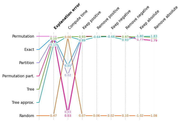
此多指标基准测试图按第一个方法对方法进行排序，并重新调整每个指标的分数以使其相对化，以便最佳分数出现在顶部，最差分数出现在底部。

shap.plots.benchmark(sum(results.values(), []))

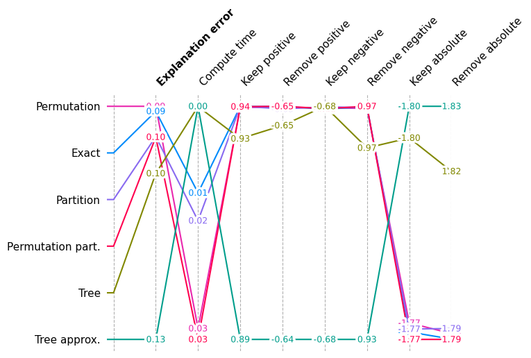
再次显示总体性能，但不包括 Random

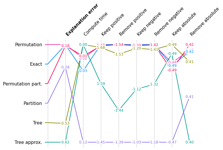
由于随机分数比合理的解释方法差得多，我们再次绘制相同的图，但不包括 Random 方法，以便我们可以看到性能方面较小的差异。

shap.plots.benchmark(filter(lambda x: x.method != "Random", sum(results.values(), [])))

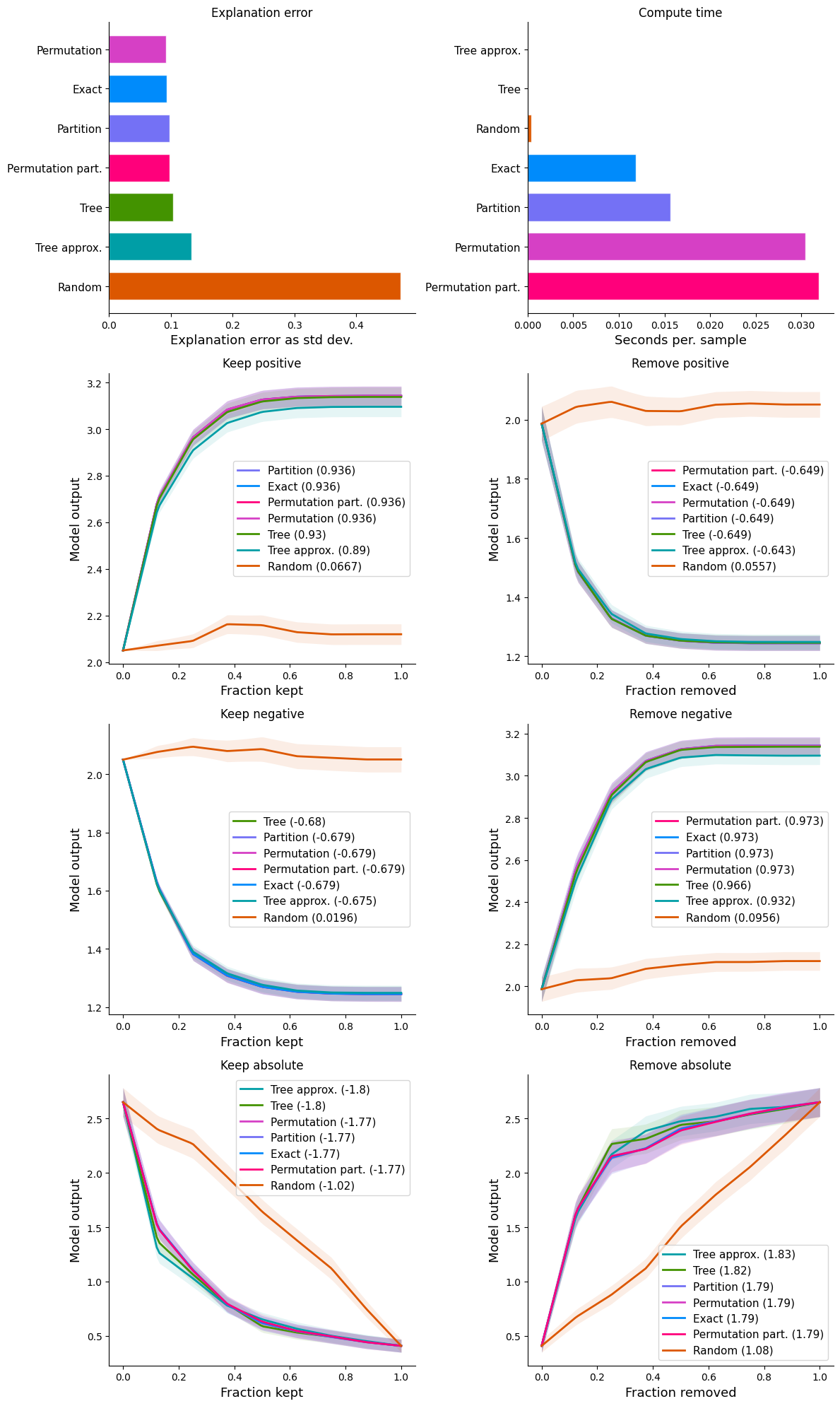
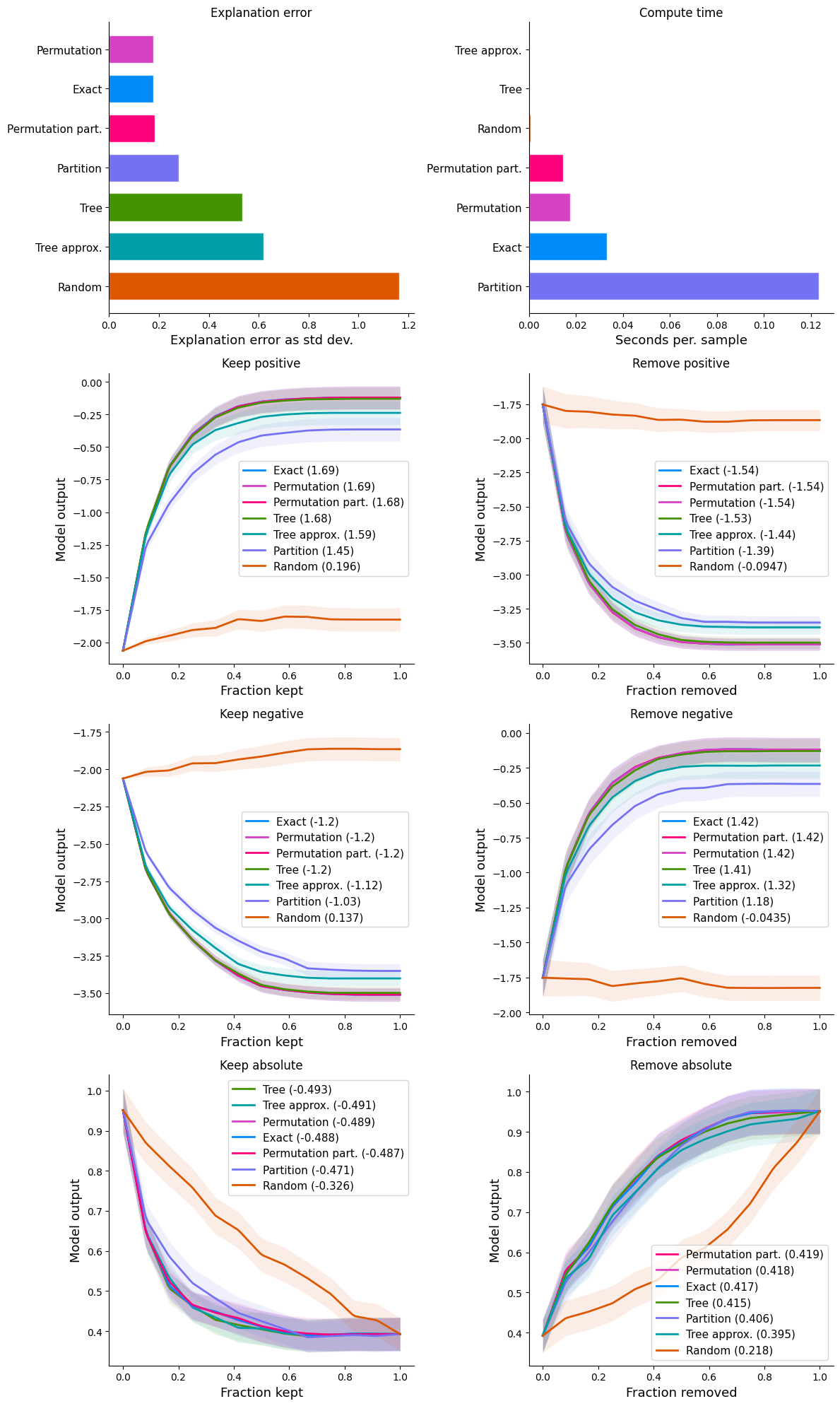
显示每种指标类型的详细图

如果我们一次绘制一个指标的分数，那么我们可以看到更详细的方法比较。一些方法只有得分（解释误差和计算时间），而其他方法则有完整的性能曲线，得分是这些曲线下（或上）的面积。

num_plot_rows = len(results) // 2 + len(results) % 2
fig, ax = plt.subplots(num_plot_rows, 2, figsize=(12, 5 * num_plot_rows))

for i, k in enumerate(results):
    plt.subplot(num_plot_rows, 2, i + 1)
    shap.plots.benchmark(results[k], show=False)
if i % 2 == 0:
    ax[-1, -1].axis("off")
plt.tight_layout()
plt.show()

在人口普查收入 XGBoost 分类模型上进行解释器基准测试

构建模型和解释

# build the model
model = xgboost.XGBClassifier(n_estimators=1000, subsample=0.3)
X, y = shap.datasets.adult(n_points=1000)
X = X.values
X_train, X_test, y_train, y_test = train_test_split(X, y, random_state=0)
model.fit(
    X_train,
    y_train,
    eval_set=[(X_test, y_test)],
    early_stopping_rounds=10,
    verbose=False,
)


def logit_predict(X):
    return model.predict(X, output_margin=True)


def loss_predict(X, y):
    probs = model.predict_proba(X)
    return [-np.log(probs[i, y[i] * 1]) for i in range(len(y))]


# define the benchmark evaluation sample set (limited to 1000 samples for the sake of time)
X_eval = X_test[:1000]
y_eval = y_test[:1000]

# use an independent masker
masker = shap.maskers.Independent(X_train)
pmasker = shap.maskers.Partition(X_train)

# build the explainers
explainers = [
    ("Permutation", shap.PermutationExplainer(logit_predict, masker)),
    ("Permutation part.", shap.PermutationExplainer(logit_predict, pmasker)),
    ("Partition", shap.PartitionExplainer(logit_predict, pmasker)),
    ("Tree", shap.TreeExplainer(model)),
    ("Tree approx.", shap.TreeExplainer(model, approximate=True)),
    ("Random", shap.explainers.other.Random(logit_predict, masker)),
    ("Exact", shap.ExactExplainer(logit_predict, masker)),
]

# # dry run to get all the code warmed up for valid runtime measurements
for name, exp in explainers:
    exp(X_eval[:1])

# explain with all the explainers
attributions = [(name, exp(X_eval)) for name, exp in explainers]

PartitionExplainer explainer: 251it [00:30,  5.34it/s]

运行基准测试

results = {}

# we run explanation error first as the primary metric
smasker = shap.benchmark.ExplanationError(masker, logit_predict, X_eval)
results["explanation error"] = [smasker(v, name=n) for n, v in attributions]

# next compute time
ct = shap.benchmark.ComputeTime()
results["compute time"] = [ct(v, name=n) for n, v in attributions]

# then removal and addition of feature metrics based on model output
for mask_type, ordering in [
    ("keep", "positive"),
    ("remove", "positive"),
    ("keep", "negative"),
    ("remove", "negative"),
]:
    smasker = shap.benchmark.SequentialMasker(mask_type, ordering, masker, logit_predict, X_eval)
    results[mask_type + " " + ordering] = [smasker(v, name=n) for n, v in attributions]

# then removal and addition of feature metrics based on model loss
cmasker = shap.maskers.Composite(masker, shap.maskers.Fixed())
for mask_type, ordering in [("keep", "absolute"), ("remove", "absolute")]:
    smasker = shap.benchmark.SequentialMasker(mask_type, ordering, cmasker, loss_predict, X_eval, y_eval)
    results[mask_type + " " + ordering] = [smasker(v, name=n) for n, v in attributions]

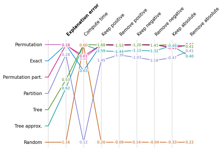
显示所有解释器的所有指标的总体曲线下面积得分

shap.plots.benchmark(sum(results.values(), []))

再次显示总体性能，但不包括 Random

shap.plots.benchmark(filter(lambda x: x.method != "Random", sum(results.values(), [])))

显示每种指标类型的详细图

num_plot_rows = len(results) // 2 + len(results) % 2
fig, ax = plt.subplots(num_plot_rows, 2, figsize=(12, 5 * num_plot_rows))

for i, k in enumerate(results):
    plt.subplot(num_plot_rows, 2, i + 1)
    shap.plots.benchmark(results[k], show=False)
if i % 2 == 0:
    ax[-1, -1].axis("off")
plt.tight_layout()
plt.show()

---

有更多有用的示例的想法吗？ 欢迎提交 Pull Request 来添加到此文档 notebook！