可解释人工智能与 Shapley 值简介
本文介绍了如何使用 Shapley 值来解释机器学习模型。Shapley 值是合作博弈论中广泛使用的方法,具有理想的属性。本教程旨在帮助您扎实理解如何计算和解释基于 Shapley 的机器学习模型解释。我们将采用实践动手的方法,使用 shap Python 包来解释越来越复杂的模型。这是一份活文档,作为 shap Python 包的介绍。因此,如果您有反馈或贡献,请打开 issue 或 pull request,以使本教程更好!
大纲
解释线性回归模型
解释广义可加回归模型
解释非可加提升树模型
解释线性逻辑回归模型
解释非可加提升树逻辑回归模型
处理相关的输入特征
解释 transformers NLP 模型
解释线性回归模型
在使用 Shapley 值解释复杂模型之前,了解它们在简单模型中的工作方式会很有帮助。最简单的模型类型之一是标准线性回归,因此下面我们在 加州住房数据集上训练线性回归模型。该数据集包含 1990 年加州各地 20,640 个街区的房屋,我们的目标是从 8 个不同的特征预测房屋中位价的自然对数
MedInc - 街区组收入中位数
HouseAge - 街区组房屋年龄中位数
AveRooms - 每户平均房间数
AveBedrms - 每户平均卧室数
Population - 街区组人口
AveOccup - 每户平均家庭成员数
Latitude - 街区组纬度
Longitude - 街区组经度
[1]:
import sklearn

import shap

# a classic housing price dataset
X, y = shap.datasets.california(n_points=1000)

X100 = shap.utils.sample(X, 100)  # 100 instances for use as the background distribution

# a simple linear model
model = sklearn.linear_model.LinearRegression()
model.fit(X, y)
[1]:
LinearRegression()
检查模型系数
理解线性模型最常见的方法是检查为每个特征学习的系数。这些系数告诉我们,当我们更改每个输入特征时,模型输出会发生多大变化
[2]:
print("Model coefficients:\n")
for i in range(X.shape[1]):
    print(X.columns[i], "=", model.coef_[i].round(5))
Model coefficients:

MedInc = 0.45769
HouseAge = 0.01153
AveRooms = -0.12529
AveBedrms = 1.04053
Population = 5e-05
AveOccup = -0.29795
Latitude = -0.41204
Longitude = -0.40125
虽然系数非常适合告诉我们当我们更改输入特征的值时会发生什么,但就其本身而言,它们并不是衡量特征总体重要性的好方法。这是因为每个系数的值都取决于输入特征的尺度。例如,如果我们要以分钟而不是年来衡量房屋的年龄,那么 HouseAge 特征的系数将变为 0.0115 / (365∗24∗60) = 2.18e-8。显然,房屋建造的年数并不比分钟数更重要,但其系数值却大得多。这意味着系数的大小不一定是衡量特征在线性模型中重要性的好方法。
使用偏依赖图获得更完整的图像
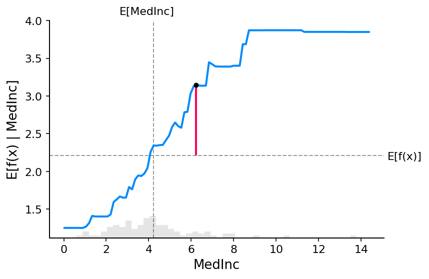
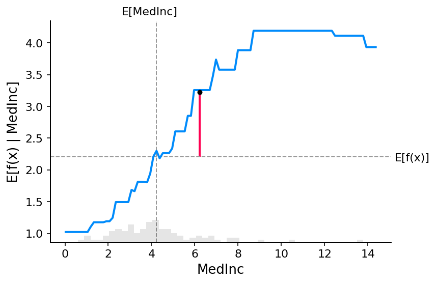
为了理解特征在模型中的重要性,有必要理解更改该特征如何影响模型的输出,以及该特征值的分布。为了可视化线性模型的这一点,我们可以构建一个经典的偏依赖图,并在 x 轴上以直方图的形式显示特征值的分布
[3]:
shap.partial_dependence_plot(
    "MedInc",
    model.predict,
    X100,
    ice=False,
    model_expected_value=True,
    feature_expected_value=True,
)
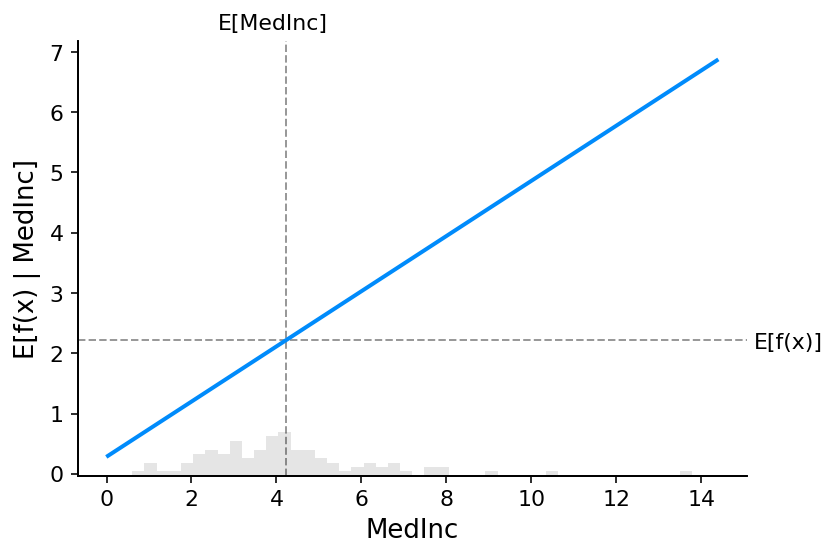
上面图中的灰色水平线表示应用于加州住房数据集时模型的期望值。垂直灰色线表示收入中位数特征的平均值。请注意,蓝色偏依赖图线(当我们修复收入中位数特征为给定值时,它是模型输出的平均值)始终穿过两条灰色期望值线的交点。我们可以将此交点视为相对于数据分布的偏依赖图的“中心”。当我们接下来转向 Shapley 值时,这种居中的影响将变得清晰。
从偏依赖图中读取 SHAP 值
基于 Shapley 值的机器学习模型解释的核心思想是使用合作博弈论中的公平分配结果,将模型输出 \(f(x)\) 的功劳分配给其输入特征。为了将博弈论与机器学习模型联系起来,有必要将模型的输入特征与博弈中的玩家匹配,并将模型函数与博弈规则匹配。由于在博弈论中,玩家可以加入或不加入博弈,因此我们需要一种方法让特征“加入”或“不加入”模型。定义特征“加入”模型含义的最常见方法是说,当我们知道该特征的值时,该特征“已加入模型”,而当我们不知道该特征的值时,该特征尚未加入模型。为了评估现有模型 \(f\),当只有特征的子集 \(S\) 是模型的一部分时,我们使用条件期望值公式积分出其他特征。此公式可以采用两种形式
或
在第一种形式中,我们知道 S 中特征的值,因为我们观察到它们。在第二种形式中,我们知道 S 中特征的值,因为我们设置了它们。一般来说,第二种形式通常更可取,因为它既告诉我们如果我们干预并更改其输入,模型将如何表现,又因为它更容易计算。在本教程中,我们将完全关注第二种公式。我们还将使用更具体的术语“SHAP 值”来指代应用于机器学习模型条件期望函数的 Shapley 值。
SHAP 值可能非常难以计算(通常是 NP-hard),但线性模型非常简单,我们可以直接从偏依赖图中读取 SHAP 值。当我们解释预测 \(f(x)\) 时,特定特征 \(i\) 的 SHAP 值只是期望模型输出与特征值 \(x_i\) 处的偏依赖图之间的差异
[4]:
# compute the SHAP values for the linear model
explainer = shap.Explainer(model.predict, X100)
shap_values = explainer(X)

# make a standard partial dependence plot
sample_ind = 20
shap.partial_dependence_plot(
    "MedInc",
    model.predict,
    X100,
    model_expected_value=True,
    feature_expected_value=True,
    ice=False,
    shap_values=shap_values[sample_ind : sample_ind + 1, :],
)
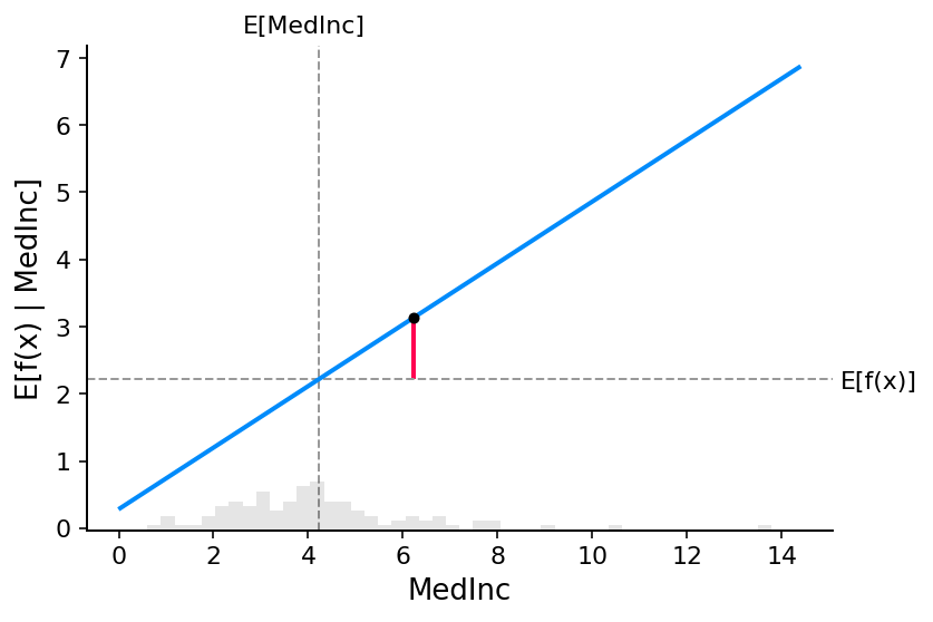
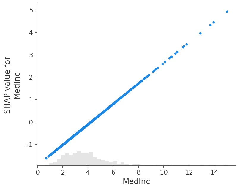
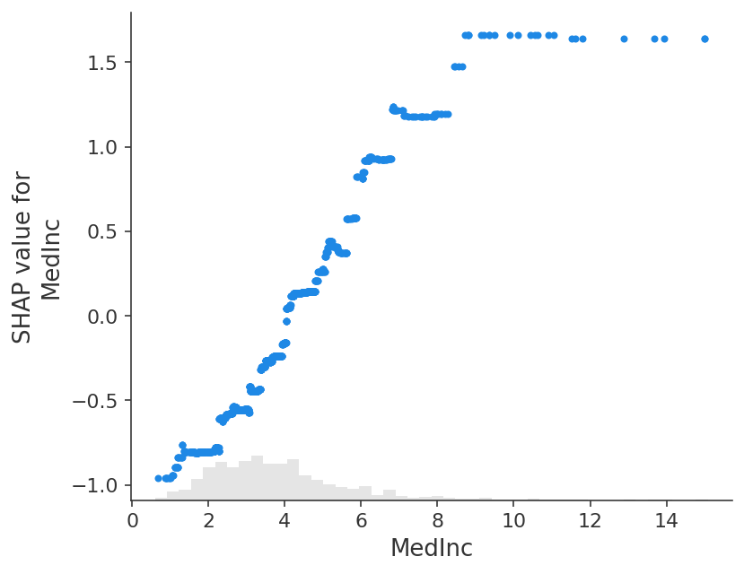
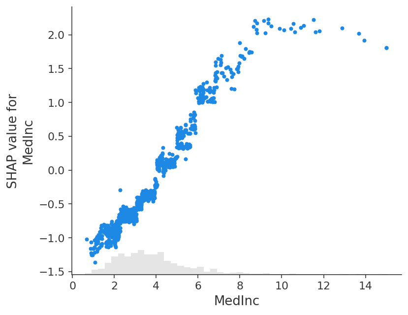
经典偏依赖图和 SHAP 值之间的紧密对应关系意味着,如果我们绘制整个数据集中特定特征的 SHAP 值,我们将完全追踪出该特征的均值中心化版本的偏依赖图
[5]:
shap.plots.scatter(shap_values[:, "MedInc"])
Shapley 值的可加性
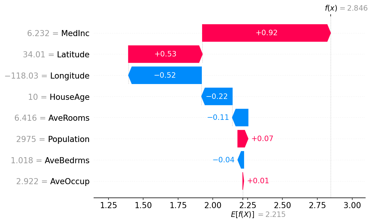
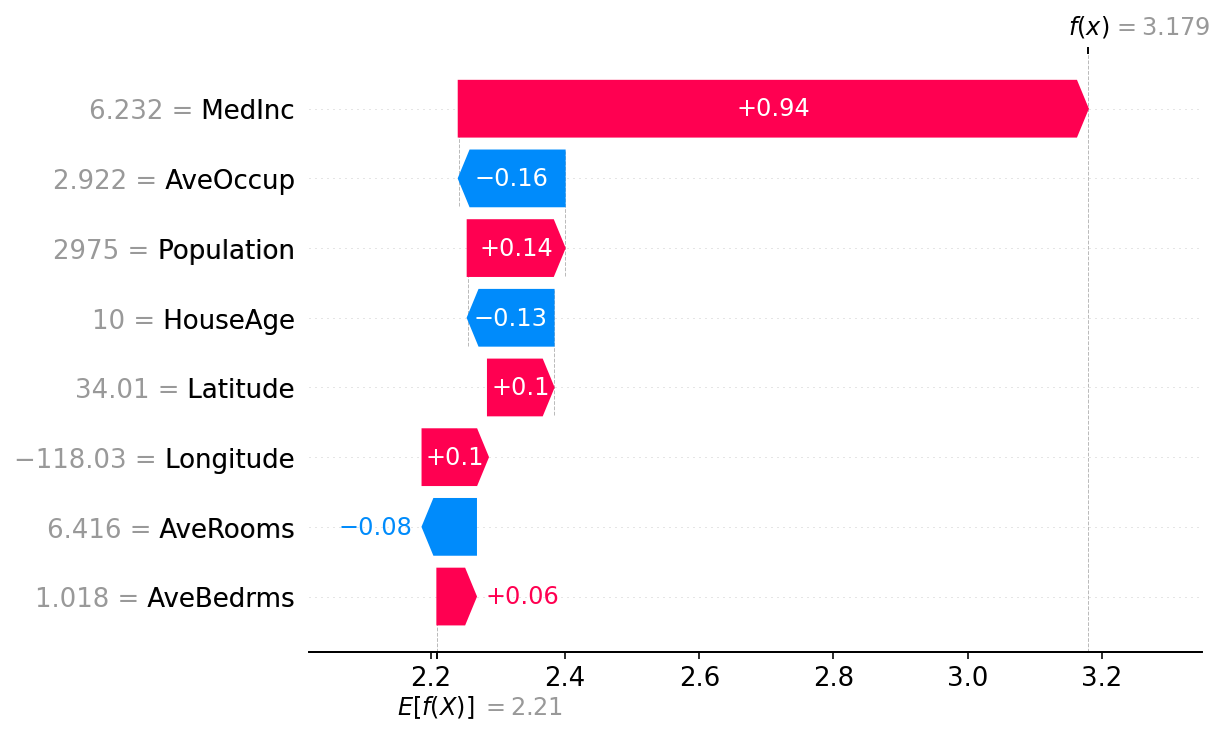
Shapley 值的基本属性之一是,当所有玩家都存在时的博弈结果与没有玩家存在时的博弈结果之间的差值始终等于所有 Shapley 值的总和。对于机器学习模型,这意味着所有输入特征的 SHAP 值将始终等于基线(期望)模型输出与被解释预测的当前模型输出之间的差值。看到这一点的最简单方法是通过瀑布图,该图从我们对房价 \(E[f(X)]\) 的背景先验期望开始,然后一次添加一个特征,直到我们达到当前模型输出 \(f(x)\)
[6]:
# the waterfall_plot shows how we get from shap_values.base_values to model.predict(X)[sample_ind]
shap.plots.waterfall(shap_values[sample_ind], max_display=14)
解释可加回归模型
线性模型的偏依赖图与 SHAP 值具有如此紧密联系的原因是,模型中的每个特征都与其他每个特征独立处理(效果只是加在一起)。我们可以保持这种可加性,同时放宽直线的线性要求。这导致了众所周知的广义可加模型 (GAM) 类。虽然有很多方法可以训练这些类型的模型(例如将 XGBoost 模型设置为深度 1),但我们将使用专门为此设计的 InterpretML 的可解释提升机。
[7]:
# fit a GAM model to the data
import interpret.glassbox

model_ebm = interpret.glassbox.ExplainableBoostingRegressor(interactions=0)
model_ebm.fit(X, y)

# explain the GAM model with SHAP
explainer_ebm = shap.Explainer(model_ebm.predict, X100)
shap_values_ebm = explainer_ebm(X)

# make a standard partial dependence plot with a single SHAP value overlaid
fig, ax = shap.partial_dependence_plot(
    "MedInc",
    model_ebm.predict,
    X100,
    model_expected_value=True,
    feature_expected_value=True,
    show=False,
    ice=False,
    shap_values=shap_values_ebm[sample_ind : sample_ind + 1, :],
)
[8]:
shap.plots.scatter(shap_values_ebm[:, "MedInc"])
[9]:
# the waterfall_plot shows how we get from explainer.expected_value to model.predict(X)[sample_ind]
shap.plots.waterfall(shap_values_ebm[sample_ind])
[10]:
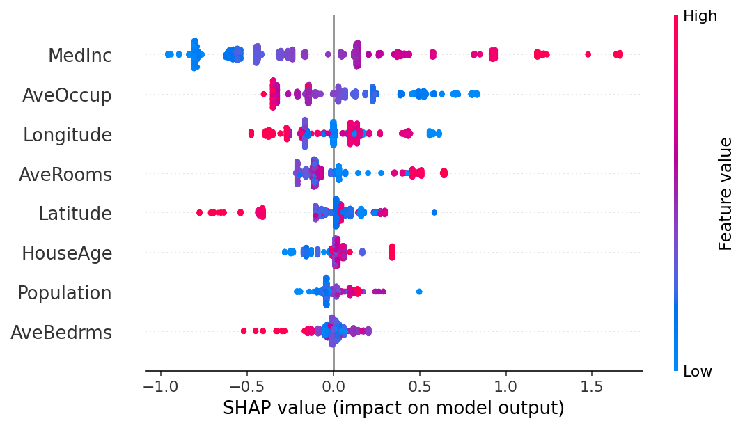
# the beeswarm plot displays SHAP values for each feature across all examples,
# with colors indicating how the SHAP values correlate with feature values
shap.plots.beeswarm(shap_values_ebm)
解释非可加提升树模型
[11]:
# train XGBoost model
import xgboost

model_xgb = xgboost.XGBRegressor(n_estimators=100, max_depth=2).fit(X, y)

# explain the GAM model with SHAP
explainer_xgb = shap.Explainer(model_xgb, X100)
shap_values_xgb = explainer_xgb(X)

# make a standard partial dependence plot with a single SHAP value overlaid
fig, ax = shap.partial_dependence_plot(
    "MedInc",
    model_xgb.predict,
    X100,
    model_expected_value=True,
    feature_expected_value=True,
    show=False,
    ice=False,
    shap_values=shap_values_xgb[sample_ind : sample_ind + 1, :],
)
[12]:
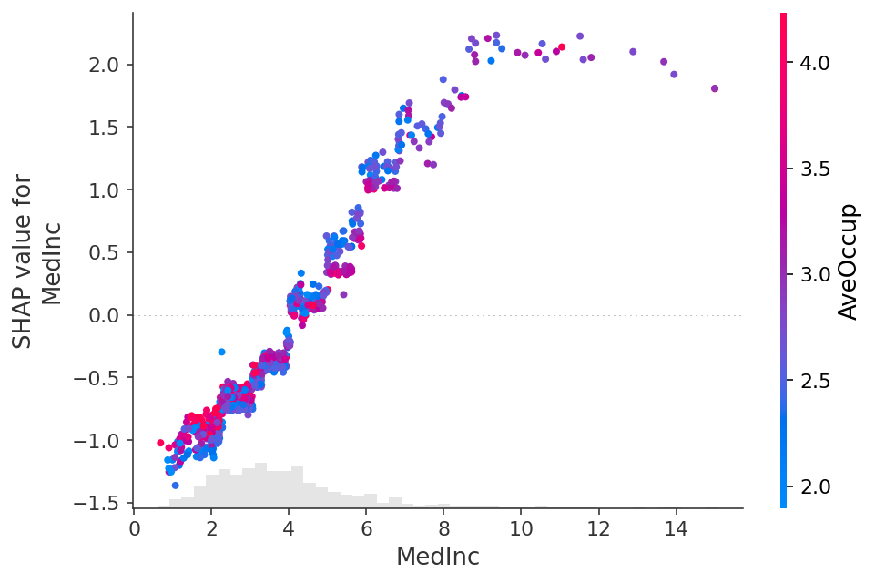
shap.plots.scatter(shap_values_xgb[:, "MedInc"])
[13]:
shap.plots.scatter(shap_values_xgb[:, "MedInc"], color=shap_values)
解释线性逻辑回归模型
[14]:
# a classic adult census dataset price dataset
X_adult, y_adult = shap.datasets.adult()

# a simple linear logistic model
model_adult = sklearn.linear_model.LogisticRegression(max_iter=10000)
model_adult.fit(X_adult, y_adult)


def model_adult_proba(x):
    return model_adult.predict_proba(x)[:, 1]


def model_adult_log_odds(x):
    p = model_adult.predict_log_proba(x)
    return p[:, 1] - p[:, 0]
请注意,解释线性逻辑回归模型的概率在输入中是非线性的。
[15]:
# make a standard partial dependence plot
sample_ind = 18
fig, ax = shap.partial_dependence_plot(
    "Capital Gain",
    model_adult_proba,
    X_adult,
    model_expected_value=True,
    feature_expected_value=True,
    show=False,
    ice=False,
)
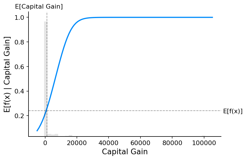
如果我们使用 SHAP 来解释线性逻辑回归模型的概率,我们会看到强大的交互作用效果。这是因为线性逻辑回归模型在概率空间中不是可加的。
[16]:
# compute the SHAP values for the linear model
background_adult = shap.maskers.Independent(X_adult, max_samples=100)
explainer = shap.Explainer(model_adult_proba, background_adult)
shap_values_adult = explainer(X_adult[:1000])
Permutation explainer: 1001it [00:58, 14.39it/s]
[17]:
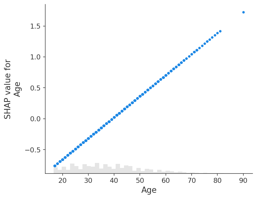
shap.plots.scatter(shap_values_adult[:, "Age"])

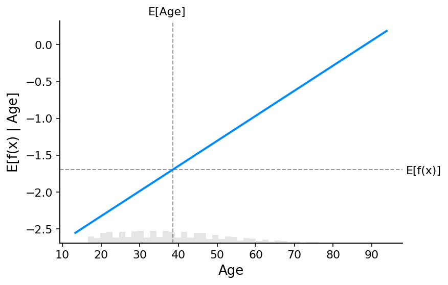
如果我们改为解释模型的对数几率输出,我们会看到模型输入和模型输出之间完美的线性关系。重要的是要记住您正在解释的模型的单位是什么,并且解释不同的模型输出可能会导致对模型行为的非常不同的看法。
[18]:
# compute the SHAP values for the linear model
explainer_log_odds = shap.Explainer(model_adult_log_odds, background_adult)
shap_values_adult_log_odds = explainer_log_odds(X_adult[:1000])
Permutation explainer: 1001it [01:01, 13.61it/s]
[19]:
shap.plots.scatter(shap_values_adult_log_odds[:, "Age"])
[20]:
# make a standard partial dependence plot
sample_ind = 18
fig, ax = shap.partial_dependence_plot(
    "Age",
    model_adult_log_odds,
    X_adult,
    model_expected_value=True,
    feature_expected_value=True,
    show=False,
    ice=False,
)
解释非可加提升树逻辑回归模型
[21]:
# train XGBoost model
model = xgboost.XGBClassifier(n_estimators=100, max_depth=2).fit(X_adult, y_adult * 1, eval_metric="logloss")

# compute SHAP values
explainer = shap.Explainer(model, background_adult)
shap_values = explainer(X_adult)

# set a display version of the data to use for plotting (has string values)
shap_values.display_data = shap.datasets.adult(display=True)[0].values
The use of label encoder in XGBClassifier is deprecated and will be removed in a future release. To remove this warning, do the following: 1) Pass option use_label_encoder=False when constructing XGBClassifier object; and 2) Encode your labels (y) as integers starting with 0, i.e. 0, 1, 2, ..., [num_class - 1].
 98%|===================| 31839/32561 [00:12<00:00]
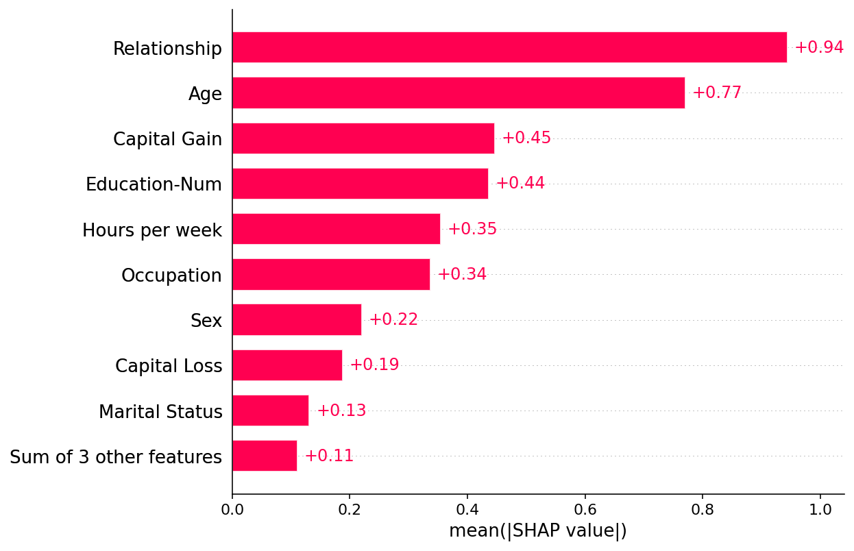
默认情况下,SHAP 条形图将取每个特征在数据集的所有实例(行)上的平均绝对值。
[22]:
shap.plots.bar(shap_values)
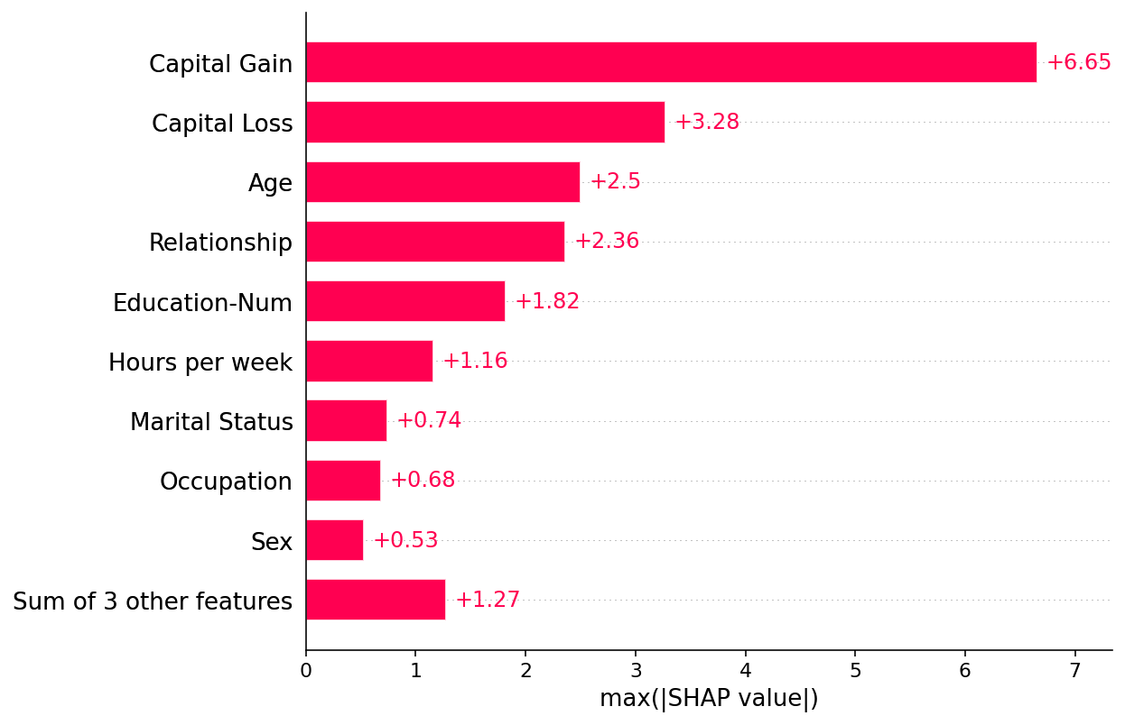
但是平均绝对值不是创建特征重要性全局度量的唯一方法,我们可以使用任意数量的变换。在这里,我们展示了如何使用最大绝对值突出显示 Capital Gain 和 Capital Loss 特征,因为它们具有不频繁但幅度大的影响。
[23]:
shap.plots.bar(shap_values.abs.max(0))
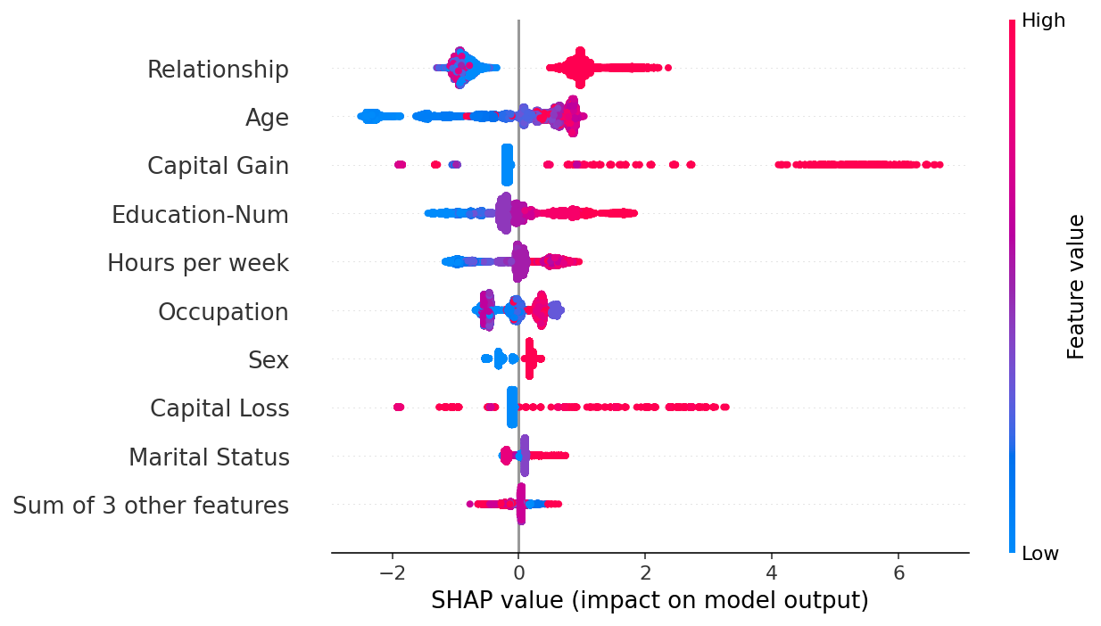
如果我们愿意处理更多的复杂性,我们可以使用蜂群图来总结每个特征的 SHAP 值的整个分布。
[24]:
shap.plots.beeswarm(shap_values)
通过取绝对值并使用纯色,我们在条形图的复杂性和完整的蜂群图之间取得了折衷。请注意,上面的条形图只是下面蜂群图中显示的值的汇总统计信息。
[25]:
shap.plots.beeswarm(shap_values.abs, color="shap_red")

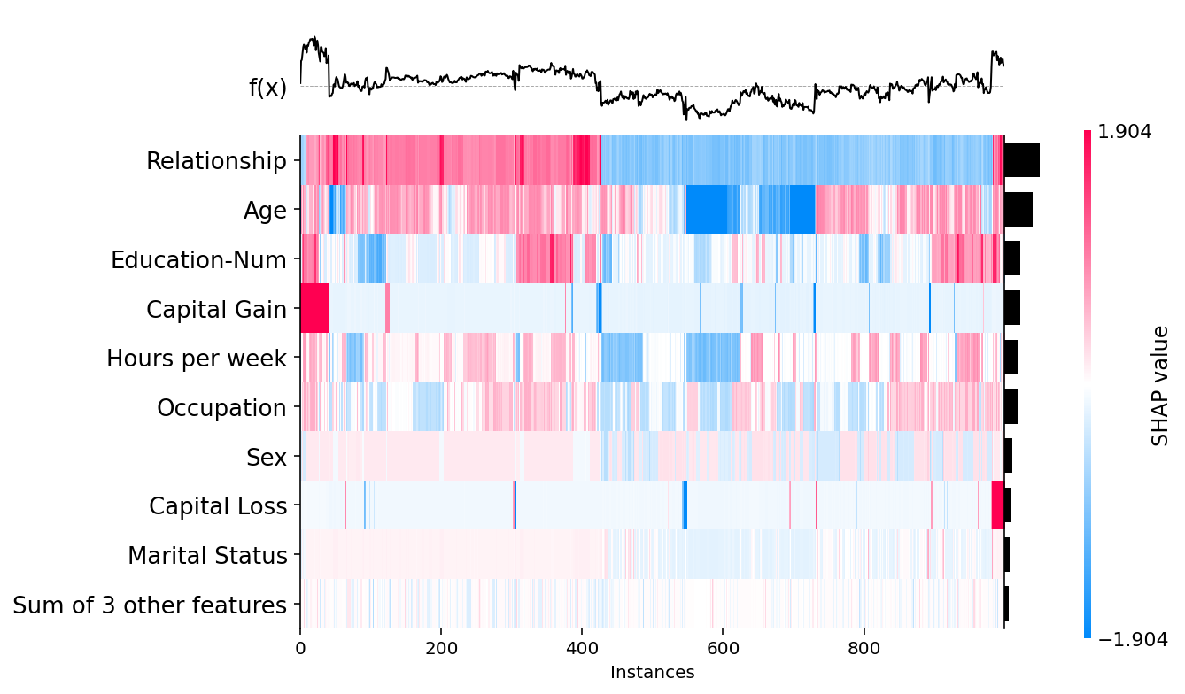
[26]:
shap.plots.heatmap(shap_values[:1000])
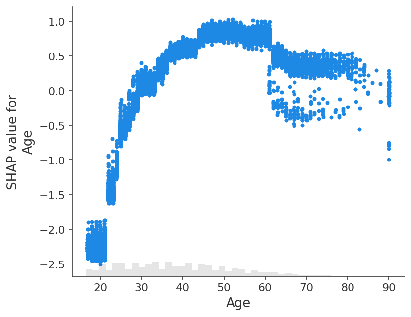
[27]:
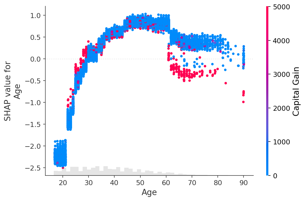
shap.plots.scatter(shap_values[:, "Age"])
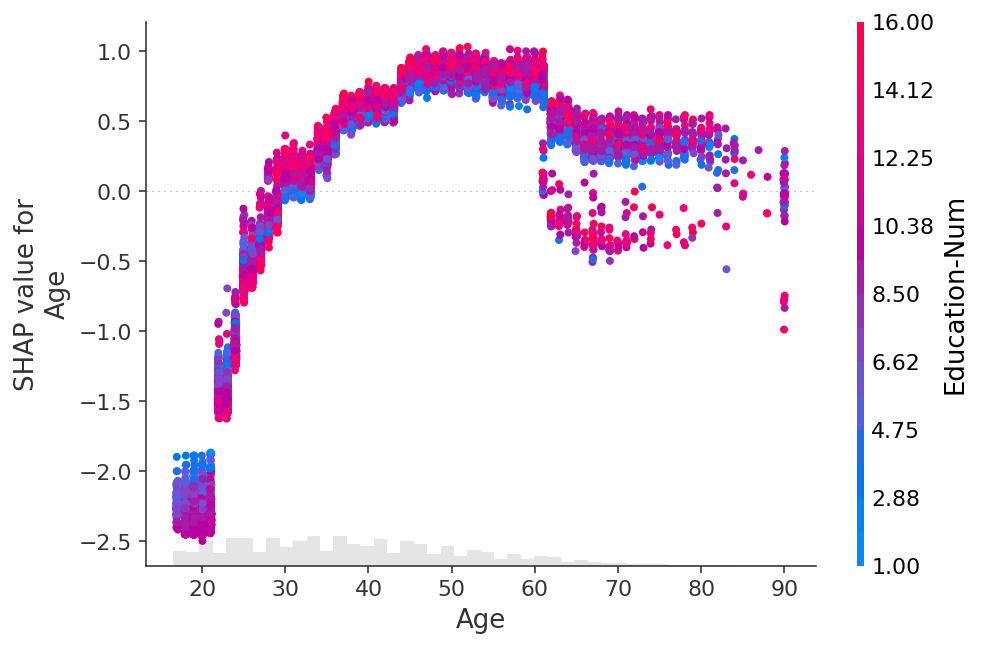
[28]:
shap.plots.scatter(shap_values[:, "Age"], color=shap_values)
[29]:
shap.plots.scatter(shap_values[:, "Age"], color=shap_values[:, "Capital Gain"])
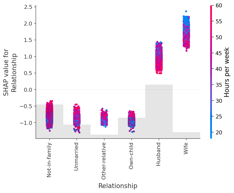
[30]:
shap.plots.scatter(shap_values[:, "Relationship"], color=shap_values)
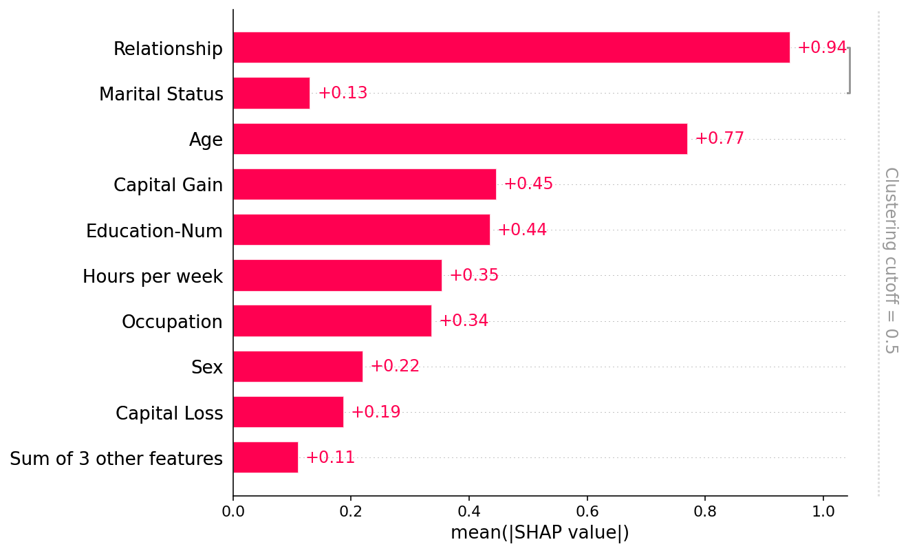
处理相关特征
[31]:
clustering = shap.utils.hclust(X_adult, y_adult)
[32]:
shap.plots.bar(shap_values, clustering=clustering)
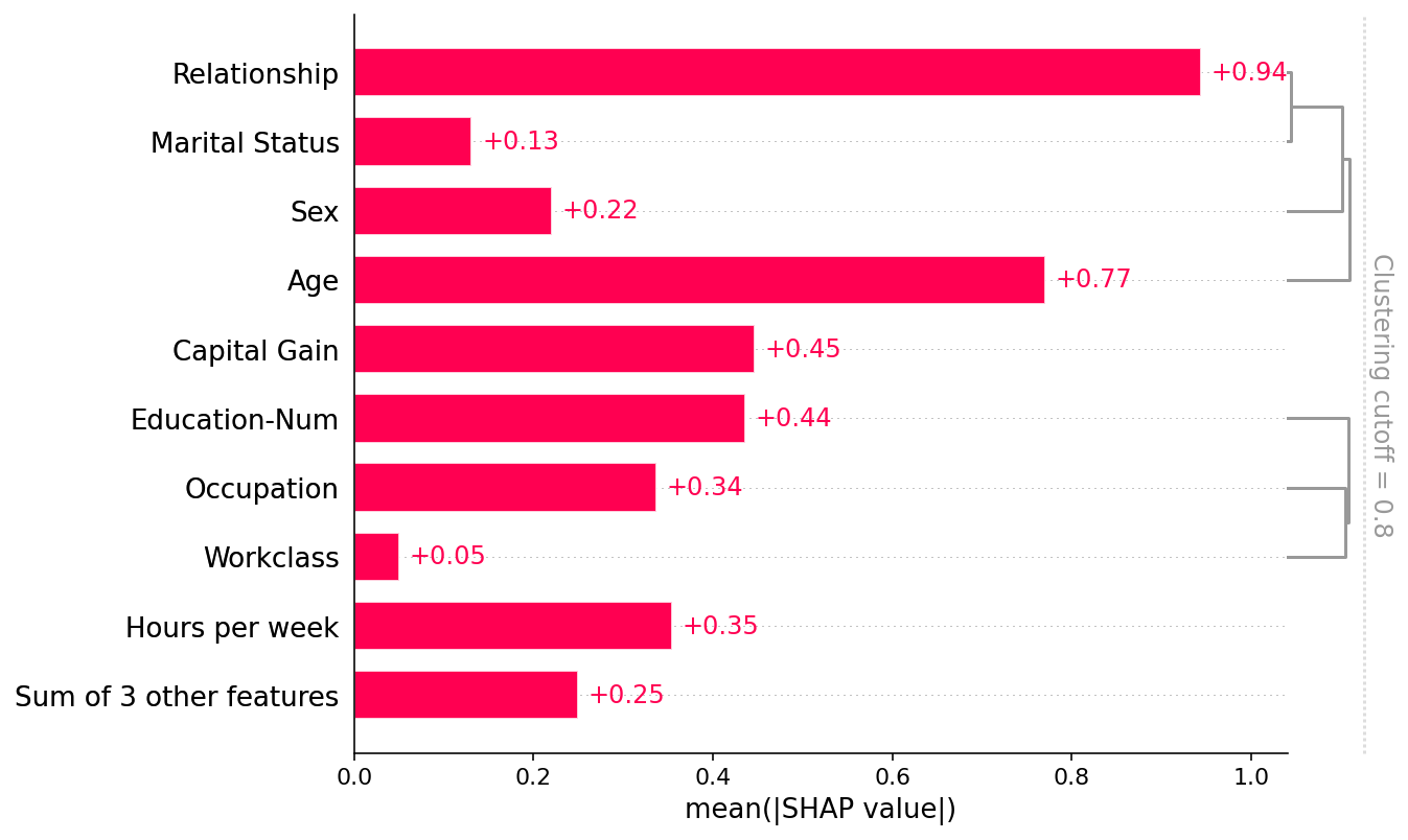
[33]:
shap.plots.bar(shap_values, clustering=clustering, clustering_cutoff=0.8)
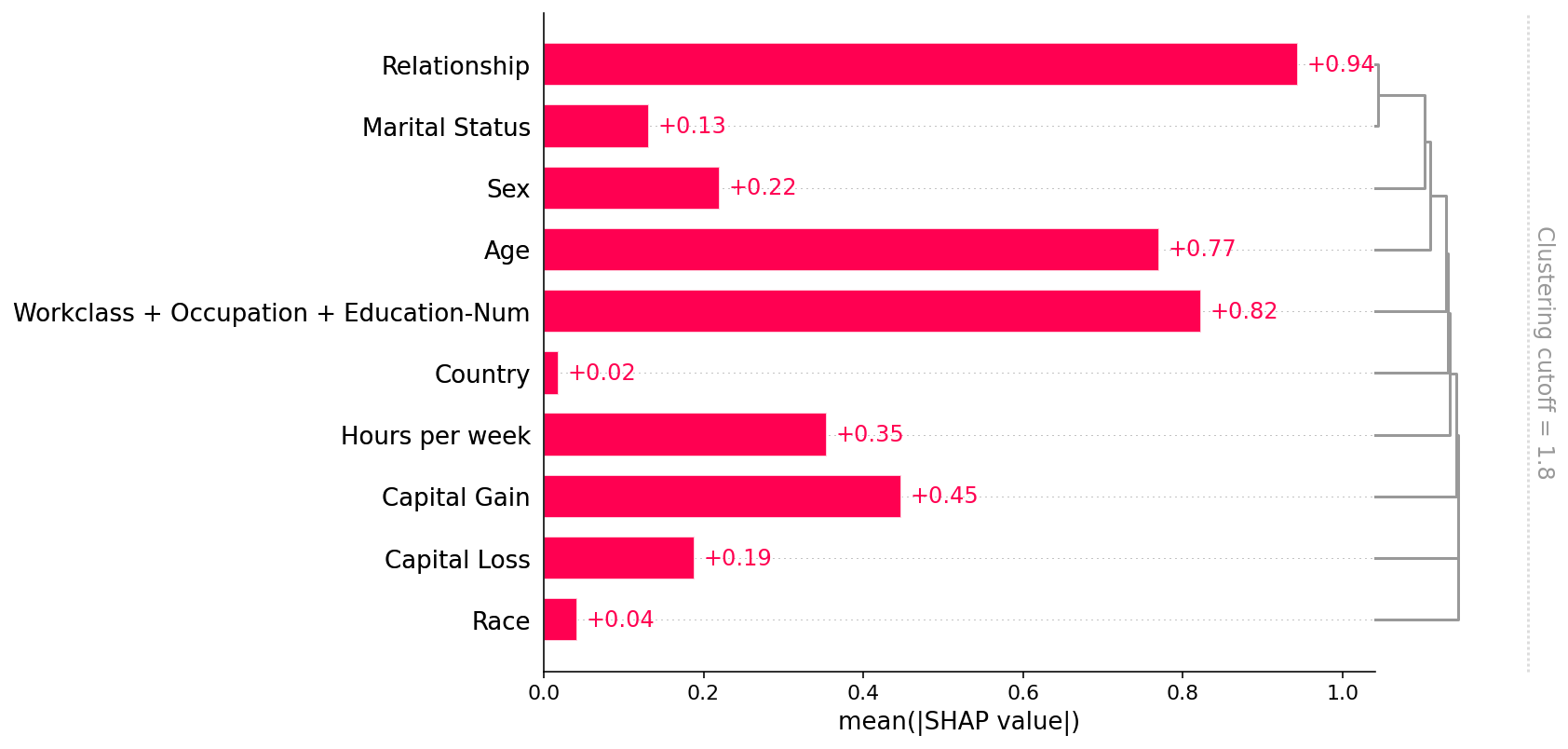
[34]:
shap.plots.bar(shap_values, clustering=clustering, clustering_cutoff=1.8)
解释 transformers NLP 模型
这演示了如何将 SHAP 应用于具有高度结构化输入的复杂模型类型。
[35]:
import datasets
import numpy as np
import scipy as sp
import torch
import transformers

# load a BERT sentiment analysis model
tokenizer = transformers.DistilBertTokenizerFast.from_pretrained("distilbert-base-uncased")
model = transformers.DistilBertForSequenceClassification.from_pretrained(
    "distilbert-base-uncased-finetuned-sst-2-english"
).cuda()


# define a prediction function
def f(x):
    tv = torch.tensor([tokenizer.encode(v, padding="max_length", max_length=500, truncation=True) for v in x]).cuda()
    outputs = model(tv)[0].detach().cpu().numpy()
    scores = (np.exp(outputs).T / np.exp(outputs).sum(-1)).T
    val = sp.special.logit(scores[:, 1])  # use one vs rest logit units
    return val


# build an explainer using a token masker
explainer = shap.Explainer(f, tokenizer)

# explain the model's predictions on IMDB reviews
imdb_train = datasets.load_dataset("imdb")["train"]
shap_values = explainer(imdb_train[:10], fixed_context=1, batch_size=2)
2022-06-15 14:43:09.022292: I tensorflow/core/platform/cpu_feature_guard.cc:142] This TensorFlow binary is optimized with oneAPI Deep Neural Network Library (oneDNN) to use the following CPU instructions in performance-critical operations:  AVX2 AVX512F FMA
To enable them in other operations, rebuild TensorFlow with the appropriate compiler flags.
2022-06-15 14:43:09.731330: I tensorflow/core/common_runtime/gpu/gpu_device.cc:1510] Created device /job:localhost/replica:0/task:0/device:GPU:0 with 8395 MB memory:  -> device: 0, name: NVIDIA GeForce RTX 2080 Ti, pci bus id: 0000:15:00.0, compute capability: 7.5
2022-06-15 14:43:09.732184: I tensorflow/core/common_runtime/gpu/gpu_device.cc:1510] Created device /job:localhost/replica:0/task:0/device:GPU:1 with 9631 MB memory:  -> device: 1, name: NVIDIA GeForce RTX 2080 Ti, pci bus id: 0000:21:00.0, compute capability: 7.5
Reusing dataset imdb (/home/slundberg/.cache/huggingface/datasets/imdb/plain_text/1.0.0/2fdd8b9bcadd6e7055e742a706876ba43f19faee861df134affd7a3f60fc38a1)
Partition explainer: 9it [00:25,  2.80s/it]Token indices sequence length is longer than the specified maximum sequence length for this model (720 > 512). Running this sequence through the model will result in indexing errors
Partition explainer: 11it [00:33,  4.21s/it]
[36]:
# plot a sentence's explanation
shap.plots.text(shap_values[2])
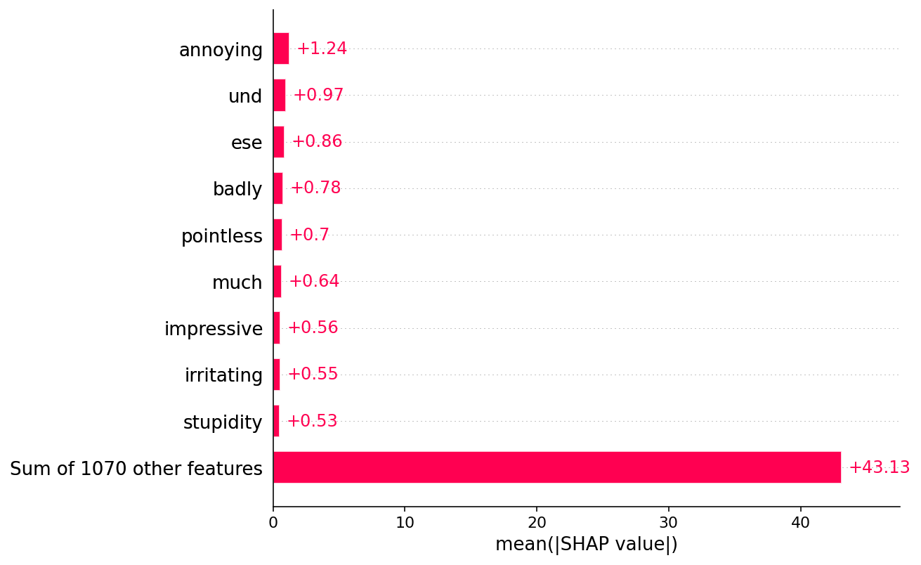
[37]:
shap.plots.bar(shap_values.abs.mean(0))
Creating an ndarray from ragged nested sequences (which is a list-or-tuple of lists-or-tuples-or ndarrays with different lengths or shapes) is deprecated. If you meant to do this, you must specify 'dtype=object' when creating the ndarray
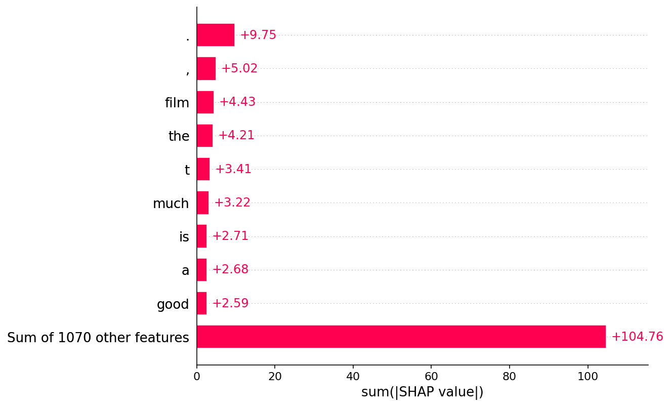
[38]:
shap.plots.bar(shap_values.abs.sum(0))
对更有帮助的示例有想法吗? 欢迎提交 pull request 来添加到此文档笔记本!