Exact 解释器

本笔记本演示了如何在一些简单数据集上使用 Exact 解释器。Exact 解释器是模型无关的，因此它可以为任何模型精确计算 Shapley 值和 Owen 值（无需近似）。然而，由于它完全枚举了掩码模式空间，因此对于 M 个输入特征，Shapley 值的复杂度为 \(O(2^M)\)，Owen 值的复杂度为 \(O(M^2)\) （在平衡聚类树上）。

因为 exact 解释器知道它正在完全枚举掩码空间，所以它可以使用随机抽样方法无法实现的优化，例如使用 格雷码 排序来最小化连续掩码模式之间变化的输入数量，从而可能减少模型需要被调用的次数。

import xgboost

import shap

# get a dataset on income prediction
X, y = shap.datasets.adult()

# train an XGBoost model (but any other model type would also work)
model = xgboost.XGBClassifier()
model.fit(X, y);

使用独立 (Shapley 值) 掩码的表格数据

# build an Exact explainer and explain the model predictions on the given dataset
explainer = shap.explainers.Exact(model.predict_proba, X)
shap_values = explainer(X[:100])

# get just the explanations for the positive class
shap_values = shap_values[..., 1]

Exact explainer: 101it [00:12,  8.13it/s]

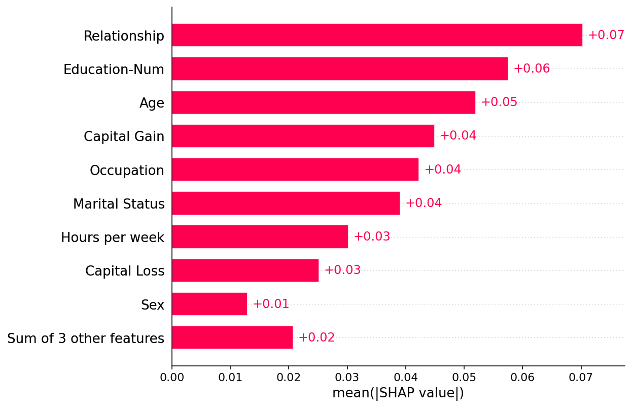
绘制全局摘要

shap.plots.bar(shap_values)

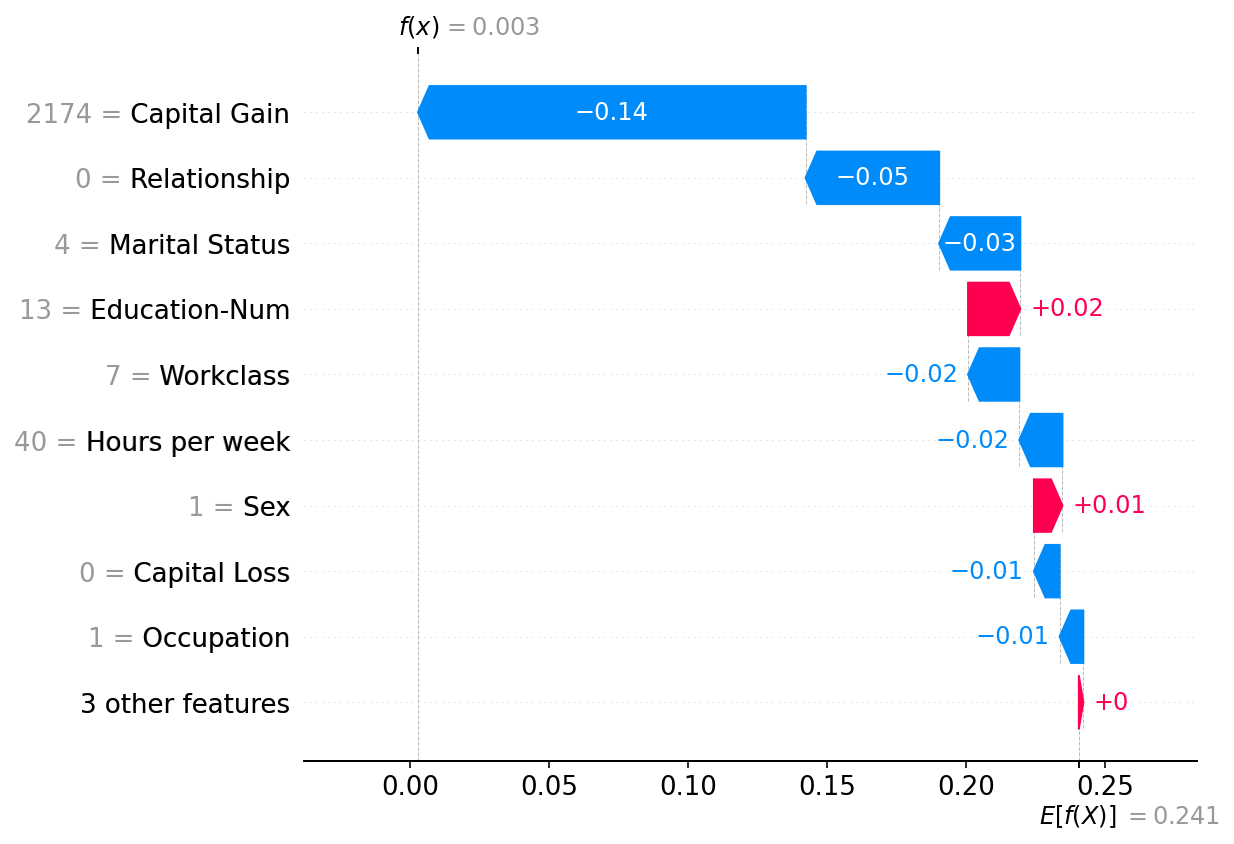
绘制单个实例

shap.plots.waterfall(shap_values[0])

使用分区 (Owen 值) 掩码的表格数据

虽然 Shapley 值是由于将每个特征与其他特征独立对待而产生的，但在模型输入上强制执行结构通常很有用。强制执行这样的结构会产生一个结构游戏（即，一个关于有效输入特征联盟规则的游戏），当该结构是一组嵌套的特征分组时，我们会得到 Owen 值，作为 Shapley 值对组的递归应用。在 SHAP 中，我们将分区推向极限，并构建一个二叉分层聚类树来表示数据的结构。这种结构可以通过多种方式选择，但对于表格数据，从输入特征之间关于输出标签的信息冗余性构建结构通常很有帮助。这正是我们在下面所做的

# build a clustering of the features based on shared information about y
clustering = shap.utils.hclust(X, y)

# above we implicitly used shap.maskers.Independent by passing a raw dataframe as the masker
# now we explicitly use a Partition masker that uses the clustering we just computed
masker = shap.maskers.Partition(X, clustering=clustering)

# build an Exact explainer and explain the model predictions on the given dataset
explainer = shap.explainers.Exact(model.predict_proba, masker)
shap_values2 = explainer(X[:100])

# get just the explanations for the positive class
shap_values2 = shap_values2[..., 1]

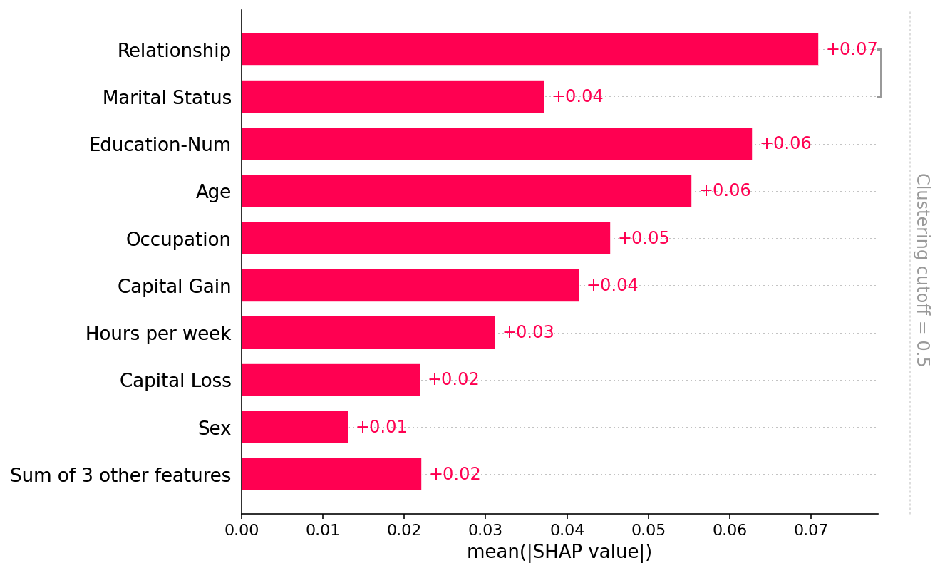
绘制全局摘要

请注意，只有 “Relationship” 和 “Marital status” 特征彼此共享超过 50% 的解释力（以 R2 衡量），因此聚类树的所有其他部分都通过默认的 clustering_cutoff=0.5 设置移除

shap.plots.bar(shap_values2)

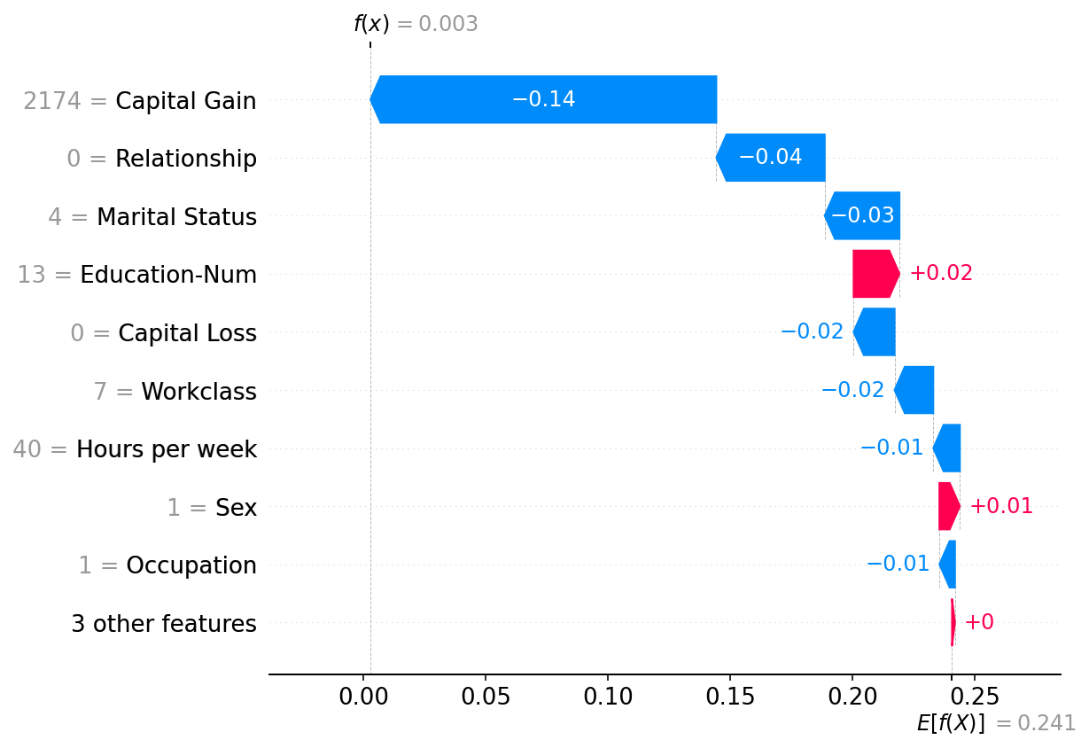
绘制单个实例

请注意，上面 Independent 掩码器和这里的 Partition 掩码器的解释之间存在很强的相似性。总的来说，对于表格数据，这些方法之间的区别不大，尽管 Partition 掩码器允许更快的运行时，并可能对模型输入进行更真实的操作（因为聚类特征组一起被掩码/取消掩码）。

shap.plots.waterfall(shap_values2[0])