多输入梯度解释器 MNIST 示例

这里我们演示了当你的 Keras/TensorFlow 模型有多个输入时，如何使用 GradientExplainer。为了保持简单但也略有趣味性，我们将 MNIST 的两个副本输入到我们的模型中，其中一个副本进入卷积网络层，另一个副本直接进入前馈网络。

import tensorflow as tf
from tensorflow.keras import Input
from tensorflow.keras.layers import Conv2D, Dense, Dropout, Flatten

# load the MNIST data
(x_train, y_train), (x_test, y_test) = tf.keras.datasets.mnist.load_data()
x_train, x_test = x_train / 255.0, x_test / 255.0
x_train = x_train.astype("float32")
x_test = x_test.astype("float32")
x_train = x_train.reshape(x_train.shape[0], 28, 28, 1)
x_test = x_test.reshape(x_test.shape[0], 28, 28, 1)

# define our model
input1 = Input(shape=(28, 28, 1))
input2 = Input(shape=(28, 28, 1))
input2c = Conv2D(32, kernel_size=(3, 3), activation="relu")(input2)
joint = tf.keras.layers.concatenate([Flatten()(input1), Flatten()(input2c)])
out = Dense(10, activation="softmax")(Dropout(0.2)(Dense(128, activation="relu")(joint)))
model = tf.keras.models.Model(inputs=[input1, input2], outputs=out)

model.compile(optimizer="adam", loss="sparse_categorical_crossentropy", metrics=["accuracy"])

# fit the model
model.fit([x_train, x_train], y_train, epochs=3)

Train on 60000 samples
Epoch 1/3
60000/60000 [==============================] - 32s 535us/sample - loss: 0.1623 - accuracy: 0.9507
Epoch 2/3
60000/60000 [==============================] - 31s 525us/sample - loss: 0.0635 - accuracy: 0.9801
Epoch 3/3
60000/60000 [==============================] - 31s 517us/sample - loss: 0.0442 - accuracy: 0.9852

<tensorflow.python.keras.callbacks.History at 0x636e08da0>

使用 GradientExplainer 解释模型所做的预测

import shap

# since we have two inputs we pass a list of inputs to the explainer
explainer = shap.GradientExplainer(model, [x_train, x_train])

# we explain the model's predictions on the first three samples of the test set
shap_values = explainer.shap_values([x_test[:3], x_test[:3]])

# since the model has 10 outputs we get a list of 10 explanations (one for each output)
print(len(shap_values))

10

# since the model has 2 inputs we get a list of 2 explanations (one for each input) for each output
print(len(shap_values[0]))

2

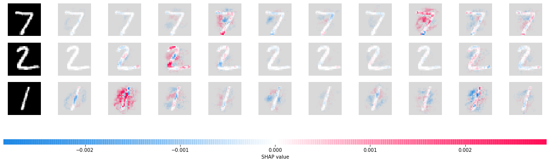
# here we plot the explanations for all classes for the first input (this is the feed forward input)
shap.image_plot([shap_values[i][0] for i in range(10)], x_test[:3])

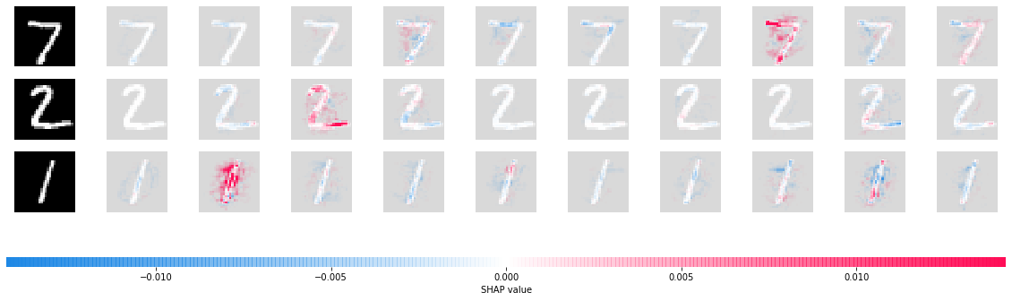
# here we plot the explanations for all classes for the second input (this is the conv-net input)
shap.image_plot([shap_values[i][1] for i in range(10)], x_test[:3])

估计抽样误差

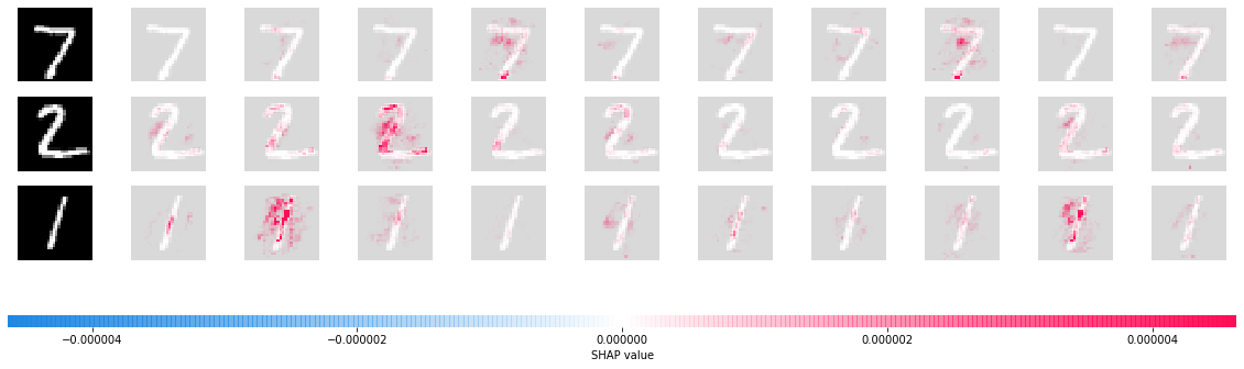
通过设置 return_variances=True，我们可以获得对解释准确性的估计。我们可以看到，使用的默认样本数（200）提供了相当低的方差估计（与上面的 shap_values 的大小相比）。请注意，您可以随时使用 nsamples 参数来控制使用的样本数。

# get the variance of our estimates
shap_values, shap_values_var = explainer.shap_values([x_test[:3], x_test[:3]], return_variances=True)

# here we plot the explanations for all classes for the first input (this is the feed forward input)
shap.image_plot([shap_values_var[i][0] for i in range(10)], x_test[:3])