简单的加州演示 2.0
本笔记演示了如何构建输入特征的层次聚类,并用它来解释单个实例。它将展示两种实现此目的的方法。
PartitionExplainer 使用您选择的 scipy 聚类方法为特征创建一个二元层次聚类。然后,PartitionExplainer 会计算遵循此二元分区树的边际特征归因。当输入特征数量较多时,这是解释单个实例的好方法。当给定一个平衡的分区树时,PartitionExplainer 的运行时复杂度为 \(O(M^2)\),其中 \(M\) 是输入特征的数量。这比 KernelExplainer 的 \(O(2^M)\) 运行时复杂度要好得多。
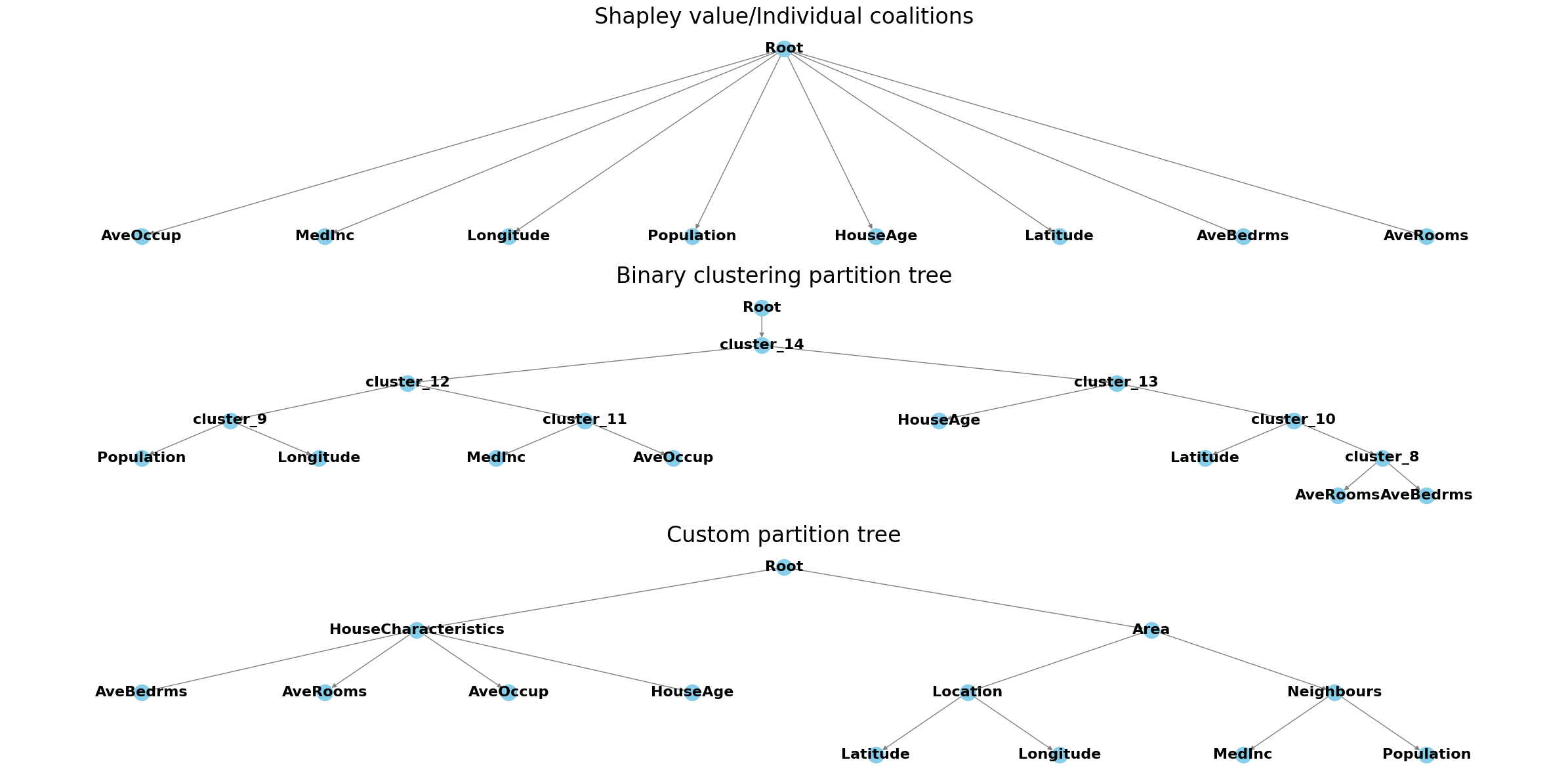
CoalitionExplainer 允许对特征的层次结构进行更多控制。用户可以以字典形式指定任何嵌套的特征层次结构。这意味着每个节点(特征组)会将其边际贡献分配给其所有兄弟节点,从而允许存在多个兄弟节点。因此,每个层级的计算复杂度为 \(O(2^K)\),其中 \(K\) 是兄弟节点的数量,具体取决于指定的特征层次结构。这种方法可以提供更合理的解释,并能对模型的工作方式进行更精细的评估。
为了澄清术语,Shapley 值将所有输入特征同等对待。Owen 值是尊重特征联盟的值。递归 Owen 值(有时也称为 Winter 值)则尊重嵌套的联盟。
[1]:
import time  # timing the methods

import matplotlib.pyplot as plt
import networkx as nx  # visualising the feature coalition structure
import numpy as np
import scipy as sp
import scipy.cluster
from xgboost import XGBRegressor  # The model we use is an XGBoost model

import shap

seed = 2023
np.random.seed(seed)
c:\programming\shap\.venv\lib\site-packages\tqdm\auto.py:21: TqdmWarning: IProgress not found. Please update jupyter and ipywidgets. See https://ipywidgets.readthedocs.io/en/stable/user_install.html
  from .autonotebook import tqdm as notebook_tqdm
训练模型
[2]:
X, y = shap.datasets.california()
model = XGBRegressor(n_estimators=100, subsample=0.3)
model.fit(X, y)

instance = X[0:1]
references = X[1:100]
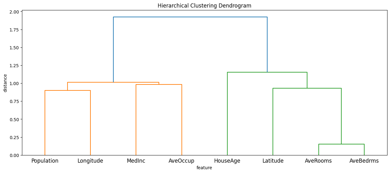
计算输入特征的层次聚类
[3]:
partition_tree = shap.utils.partition_tree(X)
plt.figure(figsize=(15, 6))
sp.cluster.hierarchy.dendrogram(partition_tree, labels=X.columns)
plt.title("Hierarchical Clustering Dendrogram")
plt.xlabel("feature")
plt.ylabel("distance")
plt.show()
解释实例
为了演示 CoalitionExplainer 的新行为并检查其是否正常工作,我们可以使用 ExactExplainer 和 PartitionExplainer 方法。
理论上,如果我们将一个扁平的层次结构传递给 CoalitionExplainer,它应该返回与 ExactExplainer 相同的结果。
如果我们将 PartitionExplainer 使用的链接矩阵转换为字典并传递给 CoalitionExplainer,它应该返回与 PartitionExplainer 完全相同的结果。
[4]:
# function to turn the linkage matrix to a dictionary
def build_partition_hierarchy(linkage, labels):
    n = len(labels)
    cluster_dict = {}

    # Initialize leaves
    for i in range(n):
        cluster_dict[i] = labels[i]

    # Build clusters
    for i, row in enumerate(linkage):
        idx1 = int(row[0])
        idx2 = int(row[1])
        cluster_id = n + i  # New cluster index

        # Create cluster names
        if idx1 < n:
            left = cluster_dict[idx1]
        else:
            left = f"cluster_{idx1}"

        if idx2 < n:
            right = cluster_dict[idx2]
        else:
            right = f"cluster_{idx2}"

        # Create the new cluster
        cluster_dict[cluster_id] = {left: cluster_dict[idx1], right: cluster_dict[idx2]}

    # The root cluster
    root_cluster_id = n + len(linkage) - 1
    return {f"cluster_{root_cluster_id}": cluster_dict[root_cluster_id]}


hierarchy_binary = build_partition_hierarchy(partition_tree, X.columns)
现在我们还可以创建一个扁平层次结构和几个非二元层次结构来测试该方法。
[5]:
# exact partition hierarchy flat
hierarchy_flat = {
    "AveOccup": "AveOccup",
    "MedInc": "MedInc",
    "Longitude": "Longitude",
    "Population": "Population",
    "HouseAge": "HouseAge",
    "Latitude": "Latitude",
    "AveBedrms": "AveBedrms",
    "AveRooms": "AveRooms",
}

# custom partition
hierarchy_nonbinary = {
    "HouseCharacteristics": {
        "AveBedrms": "AveBedrms",
        "AveRooms": "AveRooms",
        "AveOccup": "AveOccup",
        "HouseAge": "HouseAge",
    },
    "Area": {
        "Location": {"Latitude": "Latitude", "Longitude": "Longitude"},
        "Neighbours": {"MedInc": "MedInc", "Population": "Population"},
    },
}
# custom partition
hierarchy_nonbinary2 = {
    "Activity": {
        "MedInc": "MedInc",
        "AveOccup": "AveOccup",
        "Population": "Population",
    },
    "Material": {
        "AveBedrms": "AveBedrms",
        "AveRooms": "AveRooms",
        "HouseAge": "HouseAge",
    },
    "Location": {"Latitude": "Latitude", "Longitude": "Longitude"},
}
现在我们可以测试 Coalition 方法,看看它的表现如何。它在扩展 Shapley 值方法方面是否正确?与其他方法相比,它的速度表现如何?
[6]:
# Exact Shap values
start_time = time.time()
exact_explainer = shap.ExactExplainer(model.predict, X)
exact_shap_values = exact_explainer(references)
print(f"Exact Shap values computed in {time.time() - start_time:.2f} seconds")

# Tree Shap values
start_time = time.time()
tree_explainer = shap.TreeExplainer(model, X)
tree_shap_values = tree_explainer(references)
print(f"Tree Shap values computed in {time.time() - start_time:.2f} seconds")

# Old binary winter values
start_time = time.time()
masker_explainer = shap.PartitionExplainer(model.predict, X)
binary_winter_values = masker_explainer(references)
print(f"Binary Winter values computed in {time.time() - start_time:.2f} seconds")

# We can precompute the masker making the computation faster
start_time = time.time()
# build a masker from partition tree
masker = shap.maskers.Partition(X, clustering=partition_tree)
masker_explainer = shap.PartitionExplainer(model.predict, masker)
masker_winter_values = masker_explainer(references)
print(f"Binary Winter values specifying the tree computed in {time.time() - start_time:.2f} seconds")


# Shapley values corresponding to flat hierarchy
start_time = time.time()
partition_masker = shap.maskers.Partition(X)
partition_explainer_f = shap.CoalitionExplainer(model.predict, partition_masker, partition_tree=hierarchy_flat)
partition_winter_values_f = partition_explainer_f(references)
print(f"Partition Winter values (flat hierarchy) computed in {time.time() - start_time:.2f} seconds")
print(
    "The Coalition explainer recreates the ExactExplainer Shapley values:",
    np.allclose(exact_shap_values.values, partition_winter_values_f.values),
)

# Recreating the old binary winter values
start_time = time.time()

partition_explainer = shap.CoalitionExplainer(model.predict, partition_masker, partition_tree=hierarchy_binary)
partition_winter_values_b = partition_explainer(references)
print(f"Partition Winter values (binary hierarchy) computed in {time.time() - start_time:.2f} seconds")
print(
    "The Coalition explainer recreates the PartitionExplainer Winter values:",
    np.allclose(masker_winter_values.values, partition_winter_values_b.values),
)


# Shapley values for non-binary hierarchy
start_time = time.time()
partition_explainer_nb = shap.PartitionExplainer(model.predict, partition_masker, partition_tree=hierarchy_nonbinary)
partition_winter_values_nb = partition_explainer_nb(references)
print(f"Partition Winter values (non-binary hierarchy) computed in {time.time() - start_time:.2f} seconds")

# Shapley values for another non-binary hierarchy
start_time = time.time()
partition_explainer_nb2 = shap.PartitionExplainer(model.predict, partition_masker, partition_tree=hierarchy_nonbinary2)
partition_winter_values_nb2 = partition_explainer_nb2(references)
print(f"Partition Winter values (non-binary hierarchy 2) computed in {time.time() - start_time:.2f} seconds")
ExactExplainer explainer: 100it [00:10, 2.52s/it]
Exact Shap values computed in 10.06 seconds
Tree Shap values computed in 0.35 seconds
Binary Winter values computed in 4.85 seconds
Binary Winter values specifying the tree computed in 2.14 seconds
CoalitionExplainer explainer: 100it [00:24, 2.34it/s]
Partition Winter values (flat hierarchy) computed in 24.81 seconds
The Coalition explainer recreates the ExactExplainer Shapley values: True
Partition Winter values (binary hierarchy) computed in 4.98 seconds
The Coalition explainer recreates the PartitionExplainer Winter values: True
Partition Winter values (non-binary hierarchy) computed in 3.88 seconds
Partition Winter values (non-binary hierarchy 2) computed in 3.98 seconds
与 Tree SHAP 比较
[7]:
import matplotlib.pyplot as plt

plt.figure(figsize=(15, 8))

# Plot the SHAP values with enhanced visibility
plt.plot(
    exact_shap_values.values[0],
    linestyle="-",
    linewidth=2,
    label="Exact SHAP",
    color="green",
)
plt.plot(
    tree_shap_values.values[0],
    linestyle="-",
    linewidth=2,
    label="Tree SHAP",
    color="yellow",
    alpha=1,
)
plt.plot(
    binary_winter_values.values[0],
    linestyle="--",
    linewidth=2,
    label="Binary Partition SHAP",
    color="purple",
    alpha=0.6,
)
plt.plot(
    partition_winter_values_b.values[0],
    linestyle="-.",
    linewidth=2,
    label="Custom Partition SHAP",
    color="red",
    alpha=0.6,
)
plt.plot(
    partition_winter_values_b.values[0],
    linestyle="-.",
    linewidth=2,
    label="Custom Partition SHAP",
    color="blue",
    alpha=0.6,
)


# Adding title and labels with increased font sizes
plt.title("Comparison of SHAP Values", fontsize=20, fontweight="bold")
plt.xlabel("Feature Index", fontsize=16)
plt.ylabel("SHAP Value", fontsize=16)

# Customizing the legend for better readability
handles, labels = plt.gca().get_legend_handles_labels()
by_label = dict(zip(labels, handles))
plt.legend(
    by_label.values(),
    by_label.keys(),
    loc="upper right",
    fontsize=12,
    frameon=True,
    fancybox=True,
    shadow=True,
    borderpad=1,
)

# Adding a grid for better readability
plt.grid(True, which="both", linestyle="--", linewidth=0.5, alpha=0.7)

# Adding a light grey background
plt.gca().set_facecolor("whitesmoke")

# Adding a horizontal line at y=0 for reference
plt.axhline(0, color="grey", linestyle="--", linewidth=1)

# Display the plot
plt.show()
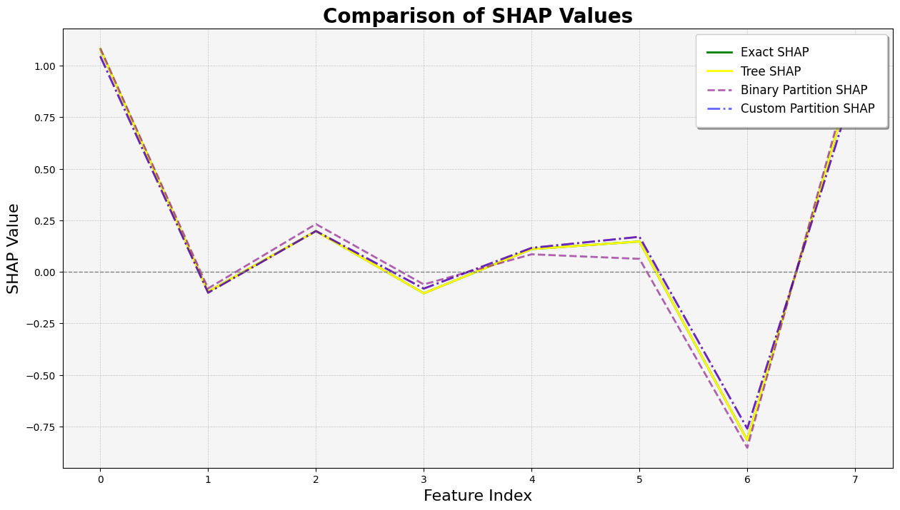
使用分区树的 Partition SHAP 值是对 SHAP 值的良好估计。分区树是减少输入特征数量和加快计算速度的好方法。
归因之所以与 Shapley 值如此接近,其原因在于,对于每个特征,其边际贡献是相对于所有其他特征被遮盖以及所有其他特征未被遮盖的情况计算的,这限定了该特征的归因范围。
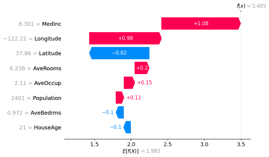
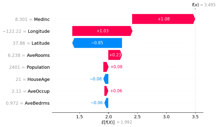
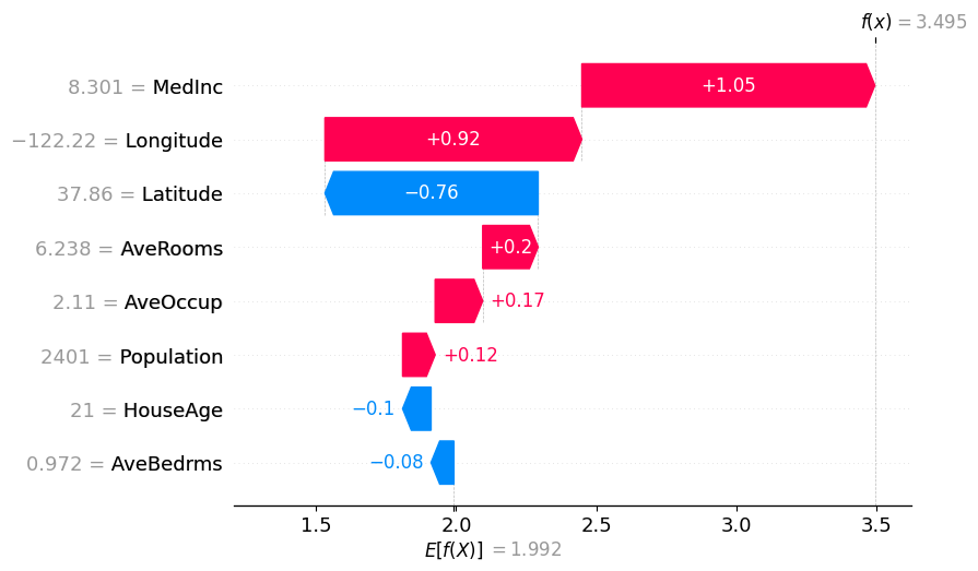
用于解释实例的图表
[8]:
# The exact Shap values
shap.plots.waterfall(exact_shap_values[0])

shap.plots.waterfall(tree_shap_values[0])

shap.plots.waterfall(partition_winter_values_f[0])  # This should match the previous


# Binary Winter values
shap.plots.waterfall(binary_winter_values[0])

# Binary Winter values specifying the partition_tree
shap.plots.waterfall(masker_winter_values[0])

# Partition Winter values (binary hierarchy but with the new method)
shap.plots.waterfall(partition_winter_values_b[0])  # This should match the previous


# Partition Winter values (non-binary hierarchy)
shap.plots.waterfall(partition_winter_values_nb[0])
# Partition Winter values (non-binary hierarchy)
shap.plots.waterfall(partition_winter_values_nb2[0])


[9]:
def add_nodes_edges(graph, parent_name, parent_dict):
    for key, value in parent_dict.items():
        if isinstance(value, dict):
            graph.add_node(key)
            graph.add_edge(parent_name, key)
            add_nodes_edges(graph, key, value)
        else:
            graph.add_node(value)
            graph.add_edge(parent_name, value)


def hierarchy_pos(G, root=None, width=1.0, vert_gap=0.2, vert_loc=0, xcenter=0.5):
    pos = _hierarchy_pos(G, root, width, vert_gap, vert_loc, xcenter)
    return pos


def _hierarchy_pos(
    G,
    root,
    width=1.0,
    vert_gap=0.2,
    vert_loc=0,
    xcenter=0.5,
    pos=None,
    parent=None,
    parsed=[],
):
    if pos is None:
        pos = {root: (xcenter, vert_loc)}
    else:
        pos[root] = (xcenter, vert_loc)

    children = list(G.neighbors(root))
    if not isinstance(G, nx.DiGraph) and parent is not None:
        children.remove(parent)

    if len(children) != 0:
        dx = width / len(children)
        nextx = xcenter - width / 2 - dx / 2
        for child in children:
            nextx += dx
            pos = _hierarchy_pos(
                G,
                child,
                width=dx,
                vert_gap=vert_gap,
                vert_loc=vert_loc - vert_gap,
                xcenter=nextx,
                pos=pos,
                parent=root,
                parsed=parsed,
            )

    return pos


fig, axes = plt.subplots(3, figsize=(24, 12))

G = nx.DiGraph()
root_name = "Root"
G.add_node(root_name)
add_nodes_edges(G, root_name, hierarchy_flat)
pos = hierarchy_pos(G, root=root_name)
nx.draw(
    G,
    pos,
    with_labels=True,
    arrows=True,
    node_size=300,
    node_color="skyblue",
    font_size=16,
    font_weight="bold",
    edge_color="gray",
    ax=axes[0],
)
axes[0].set_title("Shapley value/Individual coalitions", fontsize=24)

# Plot the first hierarchical tree
G = nx.DiGraph()
root_name = "Root"
G.add_node(root_name)
add_nodes_edges(G, root_name, hierarchy_binary)
pos = hierarchy_pos(G, root=root_name)
nx.draw(
    G,
    pos,
    with_labels=True,
    arrows=True,
    node_size=300,
    node_color="skyblue",
    font_size=16,
    font_weight="bold",
    edge_color="gray",
    ax=axes[1],
)
axes[1].set_title("Binary clustering partition tree", fontsize=24)

# Plot the second hierarchical tree
G = nx.DiGraph()
root_name = "Root"
G.add_node(root_name)
add_nodes_edges(G, root_name, hierarchy_nonbinary)
pos = hierarchy_pos(G, root=root_name)
nx.draw(
    G,
    pos,
    with_labels=True,
    arrows=True,
    node_size=300,
    node_color="skyblue",
    font_size=16,
    font_weight="bold",
    edge_color="gray",
    ax=axes[2],
)
axes[2].set_title("Custom partition tree", fontsize=24)

# Plot the third hierarchical tree


plt.tight_layout()

plt.show()
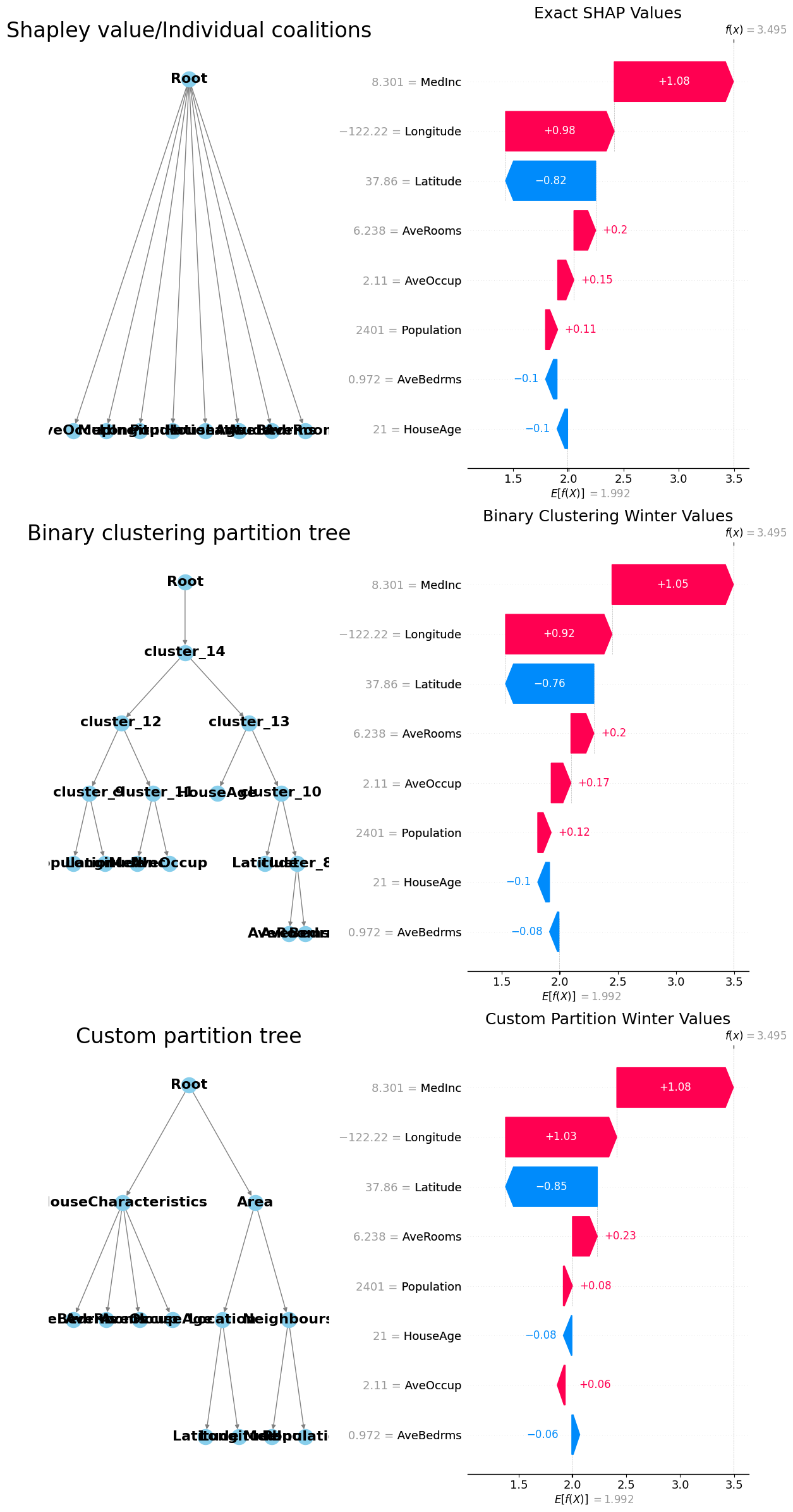
[10]:
fig, axes = plt.subplots(3, 2, figsize=(24, 36))

# Plot the first hierarchical tree
G = nx.DiGraph()
root_name = "Root"
G.add_node(root_name)
add_nodes_edges(G, root_name, hierarchy_flat)
pos = hierarchy_pos(G, root=root_name)
nx.draw(
    G,
    pos,
    with_labels=True,
    arrows=True,
    node_size=300,
    node_color="skyblue",
    font_size=16,
    font_weight="bold",
    edge_color="gray",
    ax=axes[0, 0],
)
axes[0, 0].set_title("Shapley value/Individual coalitions", fontsize=24)

# Plot the second hierarchical tree
G = nx.DiGraph()
root_name = "Root"
G.add_node(root_name)
add_nodes_edges(G, root_name, hierarchy_binary)
pos = hierarchy_pos(G, root=root_name)
nx.draw(
    G,
    pos,
    with_labels=True,
    arrows=True,
    node_size=300,
    node_color="skyblue",
    font_size=16,
    font_weight="bold",
    edge_color="gray",
    ax=axes[1, 0],
)
axes[1, 0].set_title("Binary clustering partition tree", fontsize=24)

# Plot the third hierarchical tree
G = nx.DiGraph()
root_name = "Root"
G.add_node(root_name)
add_nodes_edges(G, root_name, hierarchy_nonbinary)
pos = hierarchy_pos(G, root=root_name)
nx.draw(
    G,
    pos,
    with_labels=True,
    arrows=True,
    node_size=300,
    node_color="skyblue",
    font_size=16,
    font_weight="bold",
    edge_color="gray",
    ax=axes[2, 0],
)
axes[2, 0].set_title("Custom partition tree", fontsize=24)

# Plot the SHAP waterfall plots
plt.sca(axes[0, 1])
shap.waterfall_plot(exact_shap_values[0], show=False)
plt.gcf().set_size_inches(12, 24)
axes[0, 1].set_title("Exact SHAP Values", fontsize=18)

plt.sca(axes[1, 1])
shap.waterfall_plot(masker_winter_values[0], show=False)
plt.gcf().set_size_inches(12, 24)
axes[1, 1].set_title("Binary Clustering Winter Values", fontsize=18)

plt.sca(axes[2, 1])
shap.waterfall_plot(partition_winter_values_nb2[0], show=False)
plt.gcf().set_size_inches(12, 24)
axes[2, 1].set_title("Custom Partition Winter Values", fontsize=18)

# Adjust layout
plt.tight_layout()

# Save the figure
# plt.savefig(r'C:\Users\azabe\Documents\GitHub\Winter_values\winter_values\hierarchical_trees_and_shap_plots.png')

# Show the plot
plt.show()