使用 XGBoost 进行英雄联盟胜率预测

此笔记本使用 Kaggle 数据集英雄联盟排位赛比赛，其中包含自 2014 年开始的 180,000 场英雄联盟排位赛比赛。我们使用此数据构建 XGBoost 模型，以根据玩家在比赛中的统计数据来预测玩家的团队是否会获胜。

此处使用的方法适用于任何数据集。我们使用此数据集来说明 SHAP 值如何帮助使梯度提升树（如 XGBoost）具有可解释性。由于数据集的大小、交互效应、包含分类和连续特征以及其可解释性（特别是对于游戏玩家而言），该数据集非常适合作为各个方面的示例。有关 SHAP 值的更多信息，请参阅：https://github.com/shap/shap

from pathlib import Path

import matplotlib.pyplot as pl
import numpy as np
import pandas as pd
import xgboost as xgb
from sklearn.model_selection import train_test_split

import shap

shap.initjs()

加载数据集

要自行运行此操作，您需要从 Kaggle 下载数据集，并确保下面的 prefix 变量正确。为此，请按照上面给出的链接下载并提取数据。如果需要，更改 prefix 变量。

# read in the data
folder_path = Path("../local_scratch/data/league-of-legends-ranked-matches/")
matches = pd.read_csv(folder_path / "matches.csv")
participants = pd.read_csv(folder_path / "participants.csv")
stats1 = pd.read_csv(folder_path / "stats1.csv", low_memory=False)
stats2 = pd.read_csv(folder_path / "stats2.csv", low_memory=False)
stats = pd.concat([stats1, stats2])

# merge into a single DataFrame
a = pd.merge(participants, matches, left_on="matchid", right_on="id", suffixes=("", "_matches"))
allstats_orig = pd.merge(a, stats, left_on="matchid", right_on="id", suffixes=("", "_stats"))
allstats = allstats_orig.copy()

# drop games that lasted less than 10 minutes
allstats = allstats.loc[allstats["duration"] >= 10 * 60, :]

# Convert string-based categories to numeric values
cat_cols = ["role", "position", "version", "platformid"]
for c in cat_cols:
    allstats[c] = allstats[c].astype("category")
    allstats[c] = allstats[c].cat.codes
allstats["wardsbought"] = allstats["wardsbought"].astype(np.int32)

X = allstats.drop(columns=["win"])
y = allstats["win"]

# convert all features we want to consider as rates
rate_features = [
    "kills",
    "deaths",
    "assists",
    "killingsprees",
    "doublekills",
    "triplekills",
    "quadrakills",
    "pentakills",
    "legendarykills",
    "totdmgdealt",
    "magicdmgdealt",
    "physicaldmgdealt",
    "truedmgdealt",
    "totdmgtochamp",
    "magicdmgtochamp",
    "physdmgtochamp",
    "truedmgtochamp",
    "totheal",
    "totunitshealed",
    "dmgtoobj",
    "timecc",
    "totdmgtaken",
    "magicdmgtaken",
    "physdmgtaken",
    "truedmgtaken",
    "goldearned",
    "goldspent",
    "totminionskilled",
    "neutralminionskilled",
    "ownjunglekills",
    "enemyjunglekills",
    "totcctimedealt",
    "pinksbought",
    "wardsbought",
    "wardsplaced",
    "wardskilled",
]
for feature_name in rate_features:
    X[feature_name] /= X["duration"] / 60  # per minute rate

# convert to fraction of game
X["longesttimespentliving"] /= X["duration"]

# define friendly names for the features
full_names = {
    "kills": "Kills per min.",
    "deaths": "Deaths per min.",
    "assists": "Assists per min.",
    "killingsprees": "Killing sprees per min.",
    "longesttimespentliving": "Longest time living as % of game",
    "doublekills": "Double kills per min.",
    "triplekills": "Triple kills per min.",
    "quadrakills": "Quadra kills per min.",
    "pentakills": "Penta kills per min.",
    "legendarykills": "Legendary kills per min.",
    "totdmgdealt": "Total damage dealt per min.",
    "magicdmgdealt": "Magic damage dealt per min.",
    "physicaldmgdealt": "Physical damage dealt per min.",
    "truedmgdealt": "True damage dealt per min.",
    "totdmgtochamp": "Total damage to champions per min.",
    "magicdmgtochamp": "Magic damage to champions per min.",
    "physdmgtochamp": "Physical damage to champions per min.",
    "truedmgtochamp": "True damage to champions per min.",
    "totheal": "Total healing per min.",
    "totunitshealed": "Total units healed per min.",
    "dmgtoobj": "Damage to objects per min.",
    "timecc": "Time spent with crown control per min.",
    "totdmgtaken": "Total damage taken per min.",
    "magicdmgtaken": "Magic damage taken per min.",
    "physdmgtaken": "Physical damage taken per min.",
    "truedmgtaken": "True damage taken per min.",
    "goldearned": "Gold earned per min.",
    "goldspent": "Gold spent per min.",
    "totminionskilled": "Total minions killed per min.",
    "neutralminionskilled": "Neutral minions killed per min.",
    "ownjunglekills": "Own jungle kills per min.",
    "enemyjunglekills": "Enemy jungle kills per min.",
    "totcctimedealt": "Total crown control time dealt per min.",
    "pinksbought": "Pink wards bought per min.",
    "wardsbought": "Wards bought per min.",
    "wardsplaced": "Wards placed per min.",
    "turretkills": "# of turret kills",
    "inhibkills": "# of inhibitor kills",
    "dmgtoturrets": "Damage to turrets",
}
feature_names = [full_names.get(n, n) for n in X.columns]
X.columns = feature_names

# create train/validation split
Xt, Xv, yt, yv = train_test_split(X, y, test_size=0.2, random_state=10)
dt = xgb.DMatrix(Xt, label=yt.values)
dv = xgb.DMatrix(Xv, label=yv.values)

训练 XGBoost 模型

params = {
    "objective": "binary:logistic",
    "base_score": np.mean(yt),
    "eval_metric": "logloss",
}
model = xgb.train(
    params,
    dt,
    num_boost_round=10,
    evals=[(dt, "train"), (dv, "valid")],
    early_stopping_rounds=5,
    verbose_eval=25,
)

[0]     train-logloss:0.57255   valid-logloss:0.57258
[9]     train-logloss:0.34293   valid-logloss:0.34323

解释 XGBoost 模型

由于 Tree SHAP 算法在 XGBoost 中实现，我们可以快速计算数千个样本的精确 SHAP 值。单个预测的 SHAP 值（包括最后一列中的预期输出）总和为该预测的模型输出。

# compute the SHAP values for every prediction in the validation dataset
explainer = shap.TreeExplainer(model)
shap_values = explainer.shap_values(Xv)

解释单个玩家在特定比赛中获胜的机会

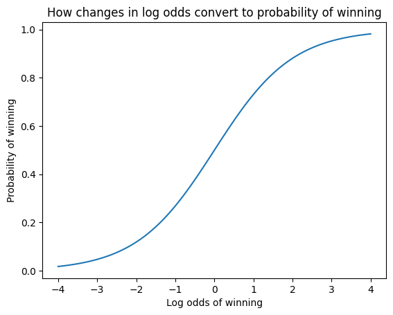
SHAP 值总和为模型的预期输出与当前玩家的当前输出之间的差值。请注意，对于 Tree SHAP 实现，解释的是模型的边际输出，而不是转换后的输出（例如逻辑回归的概率）。这意味着此模型的 SHAP 值的单位是对数几率比。较大的正值表示玩家很可能获胜，而较大的负值表示他们很可能输掉。

shap.force_plot(explainer.expected_value, shap_values[0, :], Xv.iloc[0, :])

可视化已省略，Javascript 库未加载！
您是否在此笔记本中运行了 `initjs()`？如果此笔记本来自其他用户，您还必须信任此笔记本（文件 -> 信任笔记本）。如果您在 github 上查看此笔记本，则 Javascript 已被剥离以确保安全。如果您使用的是 JupyterLab，则此错误是因为尚未编写 JupyterLab 扩展。

xs = np.linspace(-4, 4, 100)
pl.xlabel("Log odds of winning")
pl.ylabel("Probability of winning")
pl.title("How changes in log odds convert to probability of winning")
pl.plot(xs, 1 / (1 + np.exp(-xs)))
pl.show()

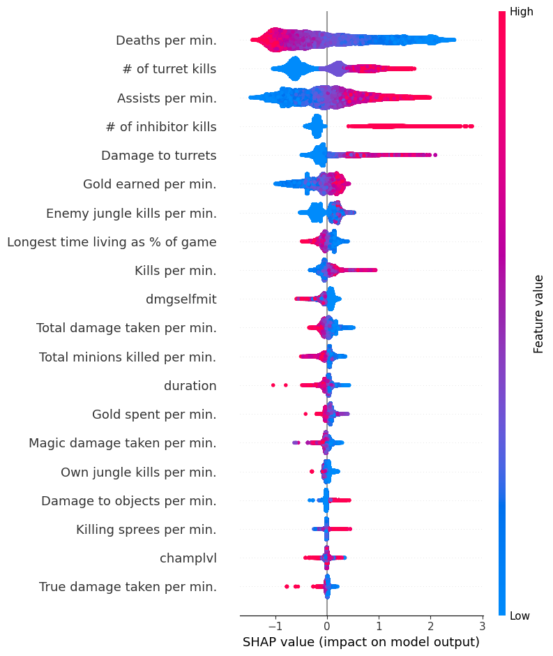
总结所有要素对整个数据集的影响

特定预测的要素的 SHAP 值表示当我们观察到该要素时模型预测的变化量。在下面的摘要图中，我们在一行中绘制单个要素（例如 goldearned）的所有 SHAP 值，其中 x 轴是 SHAP 值（对于此模型，单位为获胜的对数几率）。通过对所有要素执行此操作，我们看到哪些要素极大地驱动了模型的预测（例如 goldearned），哪些要素仅对预测产生少量影响（例如 kills）。请注意，当点在线上不适合在一起时，它们会垂直堆叠以显示密度。每个点也根据该要素的值从高到低进行着色。

shap.summary_plot(shap_values, Xv)

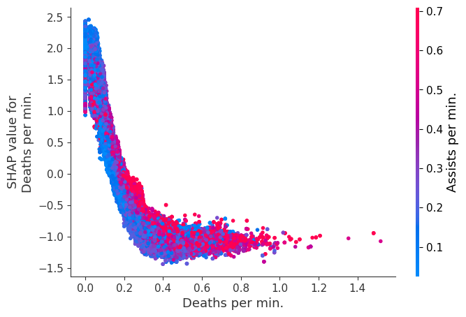
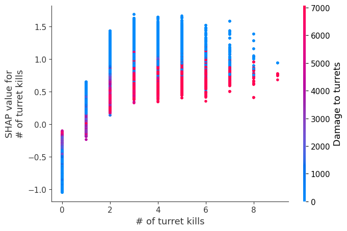
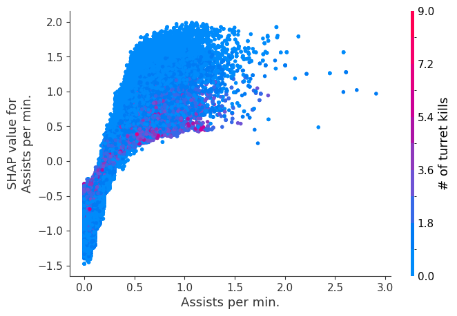
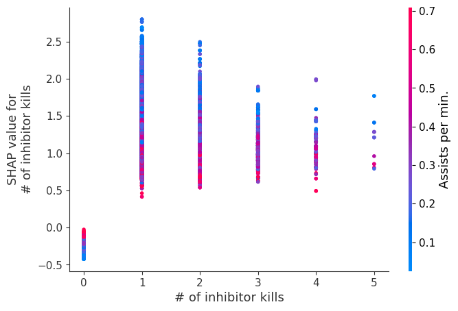
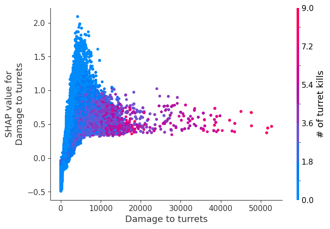
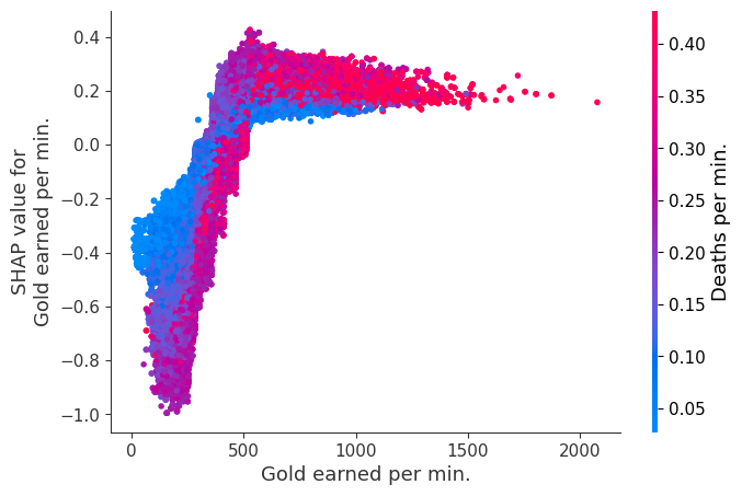
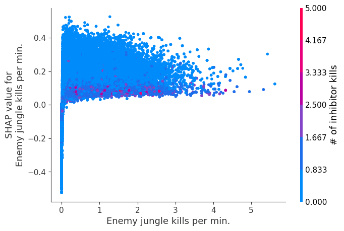
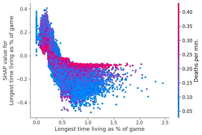
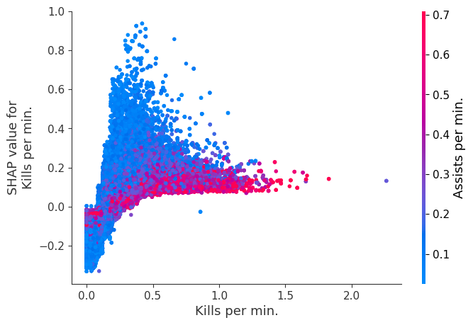
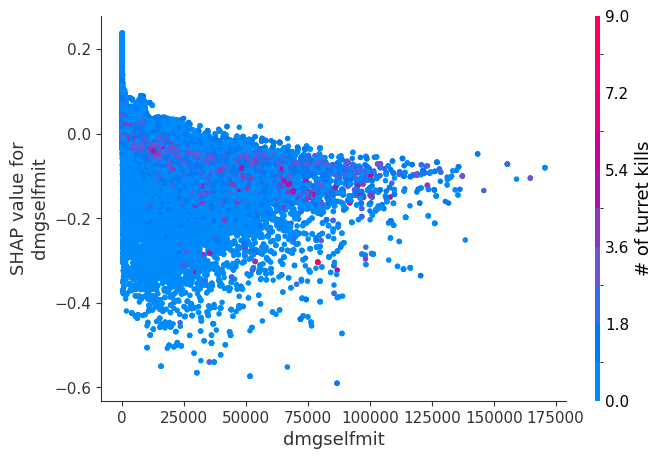
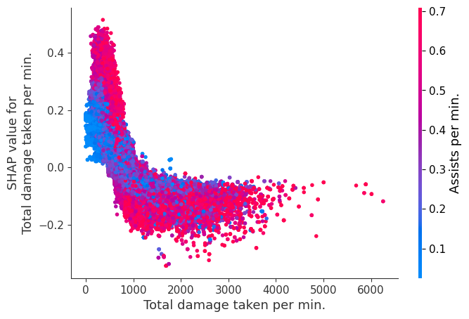
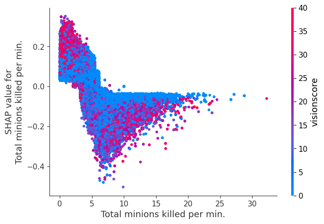
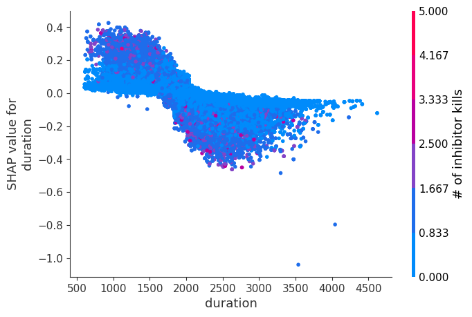
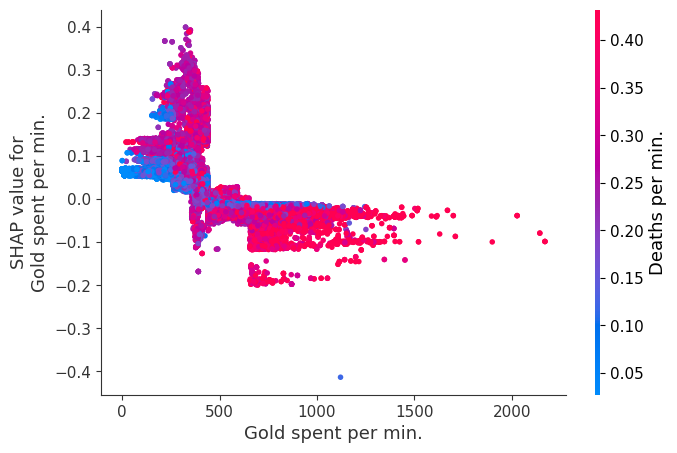
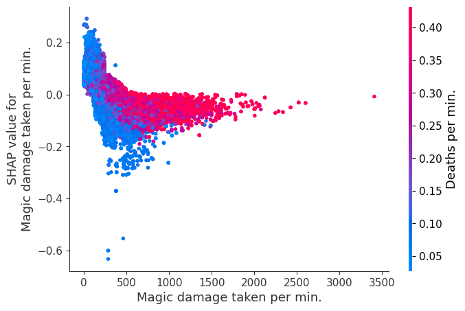
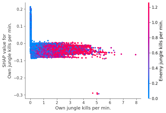
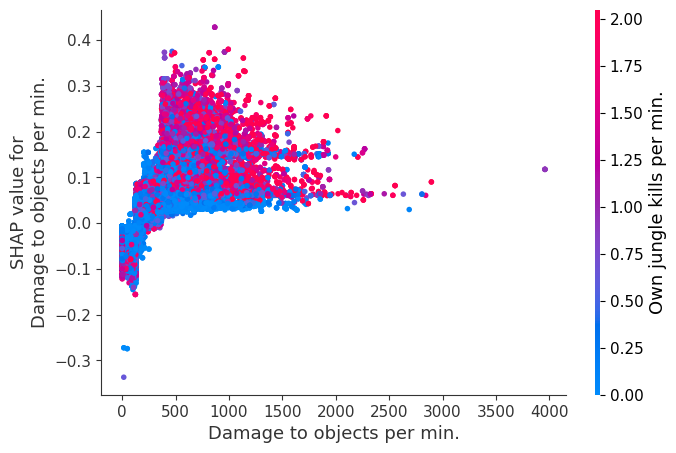
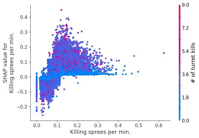
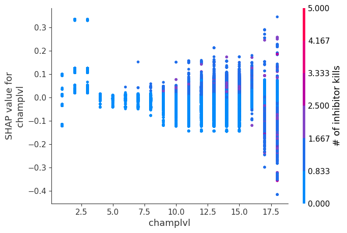
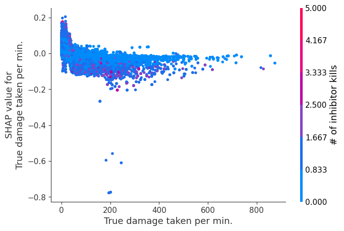
检查要素变化如何改变模型预测

我们上面训练的 XGBoost 模型非常复杂，但是通过绘制要素的 SHAP 值与所有玩家的要素实际值，我们可以看到要素值的变化如何影响模型的输出。请注意，这些图与标准部分依赖图非常相似，但是它们提供了额外的优势，即显示了上下文对于要素的重要性（或者换句话说，交互项的重要性）。交互项对要素重要性的影响程度由数据点的垂直离散度捕获。例如，在一场游戏中仅赚取 100 金币/分钟可能会使某些玩家的获胜对数几率降低 10，而另一些玩家则仅降低 3。这是为什么？因为这些玩家的其他特征会影响赚取金币对于赢得比赛的重要性。请注意，一旦您每分钟至少赚取 500 金币，垂直范围就会缩小，这意味着对于高金币赚取者而言，其他要素的上下文不如低金币赚取者重要。我们使用另一个最能解释交互效应方差的要素来为数据点着色。例如，如果您死亡次数不多，赚取较少的金币不太糟糕，但是如果您也死亡很多次，那真的很糟糕。

下图中的 y 轴表示该要素的 SHAP 值，因此 -4 表示观察到该要素会使您的获胜对数几率降低 4，而 +2 的值表示观察到该要素会使您的获胜对数几率提高 2。

请注意，这些图仅解释了 XGBoost 模型的工作原理，而不一定解释了现实的工作原理。由于 XGBoost 模型是从观察数据中训练出来的，因此它不一定是因果模型，因此仅仅因为更改某个因素会使模型对获胜的预测上升，并不总是意味着它会提高您的实际机会。

shap.dependence_plot("Gold earned per min.", shap_values, Xv, interaction_index="Deaths per min.")

# sort the features indexes by their importance in the model
# (sum of SHAP value magnitudes over the validation dataset)
top_inds = np.argsort(-np.sum(np.abs(shap_values), 0))

# make SHAP plots of the three most important features
for i in range(20):
    shap.dependence_plot(top_inds[i], shap_values, Xv)